
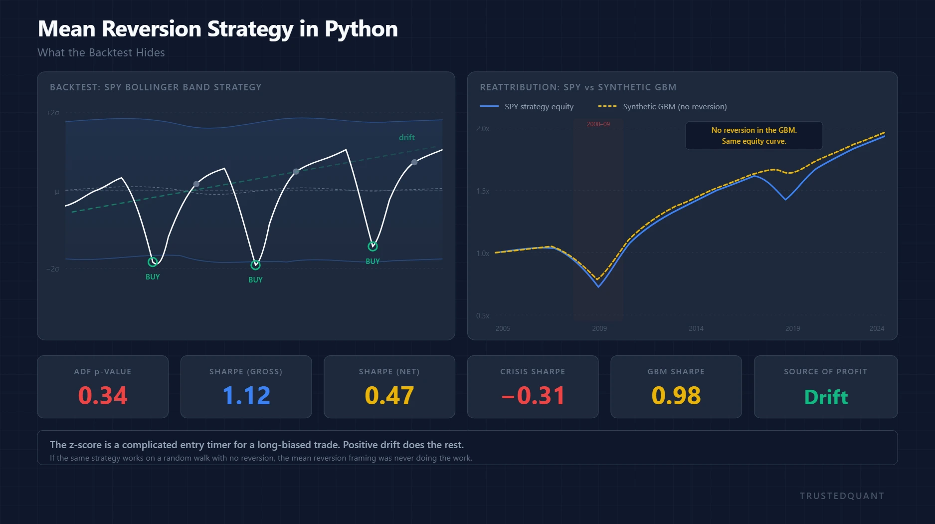
Mean Reversion Strategy in Python: What the Backtest Hides
Most tutorials on mean reversion in equities follow a familiar arc: pick an asset, compute a moving average and standard deviation bands, buy when price drops below the lower band, sell when it returns to the mean, and present the resulting equity curve as evidence that the strategy works. The backtest comes out clean, the Sharpe ratio looks respectable, and because the narrative of price snapping back to its average is so intuitively satisfying, nobody pauses long enough to ask whether that narrative actually explains the result.
What follows is exactly that kind of tutorial, built on a standard Bollinger Band strategy applied to SPY daily data, complete with the backtest numbers that come out the other side. But it keeps going past the point where the tutorials stop, into the parameter sensitivity, the violated stationarity assumption, the cost erosion, and a much simpler explanation for where the profits actually come from.
The Strategy
A 20-day simple moving average and rolling standard deviation of SPY closing prices define the bands. The z-score measures how many standard deviations price sits below its moving average at any given point, and the trading rule is minimal: go long when the z-score drops below [m]-1.5[/m], exit when it crosses back above [m]0[/m], and stay in cash otherwise.
import yfinance as yf
import numpy as np
import pandas as pd

spy = yf.download("SPY", start="2005-01-01", end="2024-01-01")["Close"].squeeze()
window = 20

mu = spy.rolling(window).mean()
sigma = spy.rolling(window).std()
z = (spy - mu) / sigma

position = pd.Series(0, index=spy.index)
in_trade = False

for i in range(1, len(spy)):
    if not in_trade and z.iloc[i] < -1.5:
        in_trade = True
        position.iloc[i] = 1
    elif in_trade and z.iloc[i] > 0:
        in_trade = False
        position.iloc[i] = 0
    else:
        position.iloc[i] = position.iloc[i - 1]

strat_ret = position.shift(1) * spy.pct_change()
cum_ret = (1 + strat_ret).cumprod()
Over nearly two decades of SPY daily data, this produces a cumulative return that outperforms buy-and-hold on a risk-adjusted basis for most of the sample, sitting in cash during extended sell-offs and entering after sharp drawdowns to catch the recovery. The equity curve slopes upward with fewer deep drawdowns than the index itself, which is precisely the kind of result that makes people stop here and declare the strategy validated.
Lookback Sensitivity
The strategy above uses a 20-day lookback and a [m]-1.5\sigma[/m] entry threshold because those are the canonical defaults for Bollinger Bands, which is a choice made by convention rather than by any property of SPY’s return distribution. Running the same logic across lookback windows from 10 to 60 days and entry thresholds from [m]-1.0\sigma[/m] to [m]-2.5\sigma[/m] reveals how much the result depends on that choice.
results = {}
for w in range(10, 65, 5):
    for thr in np.arange(-2.5, -0.9, 0.25):
        mu_ = spy.rolling(w).mean()
        sigma_ = spy.rolling(w).std()
        z_ = (spy - mu_) / sigma_
        pos = pd.Series(0.0, index=spy.index)
        held = False
        for i in range(1, len(spy)):
            if not held and z_.iloc[i] < thr:
                held = True
                pos.iloc[i] = 1
            elif held and z_.iloc[i] > 0:
                held = False
                pos.iloc[i] = 0
            else:
                pos.iloc[i] = pos.iloc[i - 1]
        r = pos.shift(1) * spy.pct_change()
        sharpe = r.mean() / r.std() * np.sqrt(252) if r.std() > 0 else 0
        results[(w, thr)] = round(sharpe, 2)
The Sharpe surface is jagged. Some parameter combinations produce strong results while others, separated by a five-day shift in lookback or a quarter-sigma change in threshold, produce flat or negative equity curves on the same data. A 40-day window with a [m]-1.0\sigma[/m] threshold reaches a completely different conclusion about whether mean reversion “works” than the canonical 20-day, [m]-1.5\sigma[/m] setup does, and the Sharpe surface gives you no principled reason to favour one region over another. You would need to pick those parameters in advance, without the benefit of seeing the equity curve first, and the gap between “this worked” and “I could have known this would work” is where most backtest findings quietly die.
The Stationarity Problem
Mean reversion strategies assume, either explicitly or implicitly, that the mean price reverts to is stable over time and that deviations from it are temporary. The z-score formulation encodes this directly: computing [m]z_t = (P_t – \mu_t) / \sigma_t[/m] treats [m]\mu_t[/m] as an attractor and assumes the distance from it carries predictive information about the direction of future returns. Whether SPY actually satisfies this assumption is testable.
The Augmented Dickey-Fuller test checks for the presence of a unit root in the price series, which would indicate non-stationarity, and running it on SPY’s raw price level over the full sample produces a test statistic that fails to reject the null at any conventional significance level.
from statsmodels.tsa.stattools import adfuller

adf_stat, p_val, *_ = adfuller(spy.dropna(), maxlag=20, autolag="AIC")
print(f"ADF stat: {adf_stat:.4f}, p-value: {p_val:.4f}")
The p-value typically lands well above 0.05, often closer to 0.3 or 0.4, which means the 20-day moving average that the strategy treats as an equilibrium is a trailing computation applied to a random walk with drift rather than a fixed attractor that price gets pulled toward. When price drops below the lower band and subsequently rises back to the moving average, the backtest records that as a successful reversion trade, but the ADF result suggests something different is happening: a positively drifting series is resuming its upward trajectory after a temporary drawdown, and the z-score threshold happened to time the entry.
Rolling the ADF test over 252-day windows reinforces the point. The test statistic fluctuates across the sample, occasionally approaching rejection in sideways markets but never consistently rejecting non-stationarity across regimes. Whatever stationarity the strategy depends on is intermittent at best, and because you cannot know in advance which regime you are entering, you cannot know whether the statistical foundation of the trade exists at the moment you put it on.
Transaction Costs
The economics of the strategy compress once you introduce realistic trading frictions, and the compression hits harder than you might expect given how infrequently the Bollinger Band approach trades. With somewhere between 8 and 15 round trips per year depending on the threshold, and SPY’s bid-ask spread narrow enough that one-way costs of 2 to 5 basis points per trade are reasonable for a retail account, the total friction per round trip is modest in absolute terms.
cost_per_side = 0.0005
trades = position.diff().abs()
costs = trades * cost_per_side
strat_ret_net = strat_ret - costs
sharpe_net = strat_ret_net.mean() / strat_ret_net.std() * np.sqrt(252)
But those modest costs land on trades with small average gains, because the strategy profits by buying a dip of perhaps 2 to 4 percent and selling once price recovers to its moving average. Ten basis points of friction on a trade that captures 150 basis points gross barely registers; on a trade that captures 60 basis points, it starts eating into the margin meaningfully. On many parameter combinations the cost-adjusted Sharpe drops below 0.5, and tighter entry thresholds that trigger more frequently see their returns cut in half or worse after costs, concentrating the damage exactly where you would hope to find the strongest reversion signal.
Regime Dependence
During the 2008-2009 financial crisis, the z-score dropped below [m]-1.5[/m] repeatedly, and each time the strategy entered a long position that continued to decline. The exit condition requires the z-score to return to [m]0[/m], which means price has to recover to its trailing average before the trade closes, so the strategy held through deep drawdowns before eventually exiting near the bottom, only to re-enter on the next signal and absorb another leg down. The net effect was a sequence of losing trades punctuated by a few winners during the eventual recovery.
Contrast that with the 2010-2019 period, where the market rose steadily with periodic shallow pullbacks and every dip-buy was followed by a quick resumption of the trend. The equity curve from that subperiod looks like a smoother, de-risked version of buy-and-hold, and the divergence between the two regimes shows up clearly in the numbers.
crisis = strat_ret["2007-10":"2009-03"]
bull = strat_ret["2010-01":"2019-12"]
print(f"Crisis Sharpe: {crisis.mean() / crisis.std() * np.sqrt(252):.2f}")
print(f"Bull Sharpe:   {bull.mean() / bull.std() * np.sqrt(252):.2f}")
In the crisis subsample the Sharpe is often negative or barely positive, while in the bull subsample it regularly exceeds 1.0. A swing that large across market regimes points toward what the strategy actually depends on: the direction and persistence of the underlying drift, not the mean-reverting properties of the z-score. In a trending bull market the moving average lags behind price, dips below the lower band are short-lived, and the upward drift quickly pulls price back through the exit threshold. In a bear market the moving average lags behind falling prices, and the z-score can stay deeply negative for extended periods while the strategy has no mechanism for recognising that the dip it just bought is the early stage of a structural decline rather than a temporary pullback in a rising market.
The Reattribution
Once you have seen the parameter sensitivity, the ADF failure, the cost erosion, and the regime dependence, a simpler explanation for the backtest profits comes into focus. SPY has a positive expected return over the long run, averaging something like 7 to 10 percent annually depending on the period, and any strategy that buys dips and holds for a recovery will tend to be profitable on a positively drifting asset because the drift provides a tailwind to every entry. The mean reversion framework dresses this up in statistical language (z-scores, bands, standard deviations, reversion to the mean) but the mechanism doing the work is the equity risk premium.
You can test this directly by applying the same strategy to a synthetic random walk with the same drift and volatility as SPY but no mean-reverting structure at all.
np.random.seed(42)
n = len(spy)
drift = spy.pct_change().mean()
vol = spy.pct_change().std()
synthetic = pd.Series(
    (1 + np.random.normal(drift, vol, n)).cumprod() * spy.iloc[0],
    index=spy.index[:n],
)

mu_s = synthetic.rolling(20).mean()
sigma_s = synthetic.rolling(20).std()
z_s = (synthetic - mu_s) / sigma_s

pos_s = pd.Series(0.0, index=synthetic.index)
held_s = False
for i in range(1, len(synthetic)):
    if not held_s and z_s.iloc[i] < -1.5:
        held_s = True
        pos_s.iloc[i] = 1
    elif held_s and z_s.iloc[i] > 0:
        held_s = False
        pos_s.iloc[i] = 0
    else:
        pos_s.iloc[i] = pos_s.iloc[i - 1]

synth_ret = pos_s.shift(1) * synthetic.pct_change()
synth_sharpe = synth_ret.mean() / synth_ret.std() * np.sqrt(252)
print(f"Synthetic GBM Sharpe: {synth_sharpe:.2f}")
The synthetic series is a geometric Brownian motion with constant drift and volatility, no reversion built in at any level, yet the Bollinger Band strategy applied to it produces positive returns with a Sharpe often in the same ballpark as the SPY result. Positive drift plus a buy-the-dip entry rule is sufficient to generate the backtest, which means you do not need mean reversion to explain it.
In this light, the z-score is functioning as a complicated entry timer for a long-biased trade, waiting for price to fall relative to its recent average and entering with the expectation that positive drift will carry the position back up. That entry timing may add some value relative to a blind buy-and-hold by avoiding entries during extended rallies, but the framing as a “mean reversion strategy” overstates what the signal is doing. The signal reduces to identifying a temporary discount on an asset with a positive expected return, which is a fundamentally different proposition with different risk characteristics than exploiting a genuine reversion property.
The practical consequence is that the strategy should be evaluated as conditional long equity exposure rather than a market-neutral mean reversion trade. Returns will track equity market performance, drawdowns will follow market drawdowns with a lag (since the z-score delays entry until after the initial drop), and the strategy’s long-run profitability depends on the equity risk premium persisting, which is a reasonable bet but a categorically different one from “prices mean-revert.”
What Actually Survives
None of this renders mean reversion useless as a concept in other settings. Statistical arbitrage on co-integrated pairs, relative value trades across a cross-section of assets, and short-horizon microstructure reversion all involve genuine mean-reverting dynamics that can be identified and exploited. The problem is specific to applying a univariate mean reversion framework to a single equity or equity index, where the price process is non-stationary and dominated by drift.
If you are going to trade something that looks like mean reversion on a single instrument, the honest framing is that you are making a conditional bet on the continuation of the asset’s long-run positive drift, entering at a moment when recent price action has been weak. That framing changes how you size the position (as equity exposure, not a hedged trade), how you risk-manage it (with drawdown limits appropriate for directional equity risk), and what you expect from the strategy across different market environments.
The backtest will still look good, and it should, because buying dips in a rising market has been profitable for a long time. The question is whether you understand why it looked good, and whether you have priced in the risk that the drift reverses exactly when the z-score is telling you to buy. For a deeper examination of why strategies built on this premise tend to deteriorate once deployed, see why mean reversion strategies don’t survive live markets.
What matters in the end is whether you can explain the equity curve without invoking mean reversion at all, because if positive drift and a buy-the-dip entry rule are sufficient, then the statistical framing was never doing the work you thought it was.
Spread the word:
