Hurst Exponent for Mean Reversion Testing

The Hurst exponent is one of the most frequently cited statistics in mean reversion research and one of the least carefully applied. Its appeal is obvious: a single number that summarizes whether a time series is trending, mean-reverting, or random. [m]H > 0.5[/m] indicates persistence, [m]H < 0.5[/m] indicates anti-persistence, and [m]H = 0.5[/m] is the boundary case of a random walk. Practitioners use it to screen pairs, filter universes, and validate spread constructions before committing capital.

The problem is that “the Hurst exponent” is not a single estimator. At least four methods are in common use, and they routinely disagree with each other on the same data. Rescaled range analysis, detrended fluctuation analysis, variance of lagged differences, and the generalised Hurst exponent each define and measure self-similarity through different lenses. Running all four on an equity spread and averaging the results, as some practitioners do, produces a number that inherits every method’s bias while cancelling none of them.

Understanding why these methods diverge matters more than knowing which one to run. Each estimator carries assumptions about the data-generating process, each interacts differently with finite-sample bias and lag selection, and each fails in specific ways that can push a marginal series across the [m]H = 0.5[/m] boundary in either direction. A spread that looks mean-reverting under R/S analysis can look persistent under DFA, and both results can be correct in the narrow sense that each estimator is answering a different question about the structure of the series.

Rescaled Range Analysis and Its Reputation Problem

Rescaled range analysis is the oldest method, introduced by Hurst himself for Nile flood data and later formalized by Mandelbrot. The procedure divides the series into blocks of length [m]n[/m], computes the range of cumulative deviations from the block mean, rescales by the standard deviation, and estimates [m]H[/m] from the power-law relationship between the rescaled range and [m]n[/m].

R/S has a well-documented upward bias. For a pure random walk, it consistently estimates [m]H[/m] above 0.5, typically in the range 0.55 to 0.65 depending on series length. The bias is structural: rescaled range statistics are sensitive to short-range autocorrelation, and even weak serial dependence inflates the estimate. For a practitioner screening pairs, this means R/S will systematically make random spreads look persistent and mean-reverting spreads look closer to random than they are.

Lo’s modified R/S statistic was designed to correct for this by adjusting the denominator with a Newey-West style long-run variance estimator. The correction helps, but introduces a new problem: the bandwidth parameter for the long-run variance estimate has to be chosen, and the choice matters. Too narrow a bandwidth underestimates long-range dependence and leaves the bias partially intact. Too wide a bandwidth inflates the variance of the estimator and drowns the signal. There is no principled way to set this parameter without already knowing the dependence structure you are trying to estimate.

The practical consequence is that R/S, even in its modified form, is unreliable as a standalone screen for mean reversion. It remains useful as an initial sanity check, partly because its biases are well understood and partly because it is robust to distributional assumptions that trip up other methods. A series that shows [m]H < 0.5[/m] under R/S, despite the method’s upward bias, is telling you something genuine. A series that shows [m]H = 0.55[/m] under R/S is telling you almost nothing.

Detrended Fluctuation Analysis Answers a Different Question

DFA was developed in the biophysics literature to handle non-stationary series, and it arrived in quantitative finance with that pedigree largely unexamined. The method works by dividing the series into windows, fitting a polynomial trend within each window, computing the root-mean-square fluctuation of the residuals, and extracting the scaling exponent [m]\alpha[/m] from the log-log relationship between fluctuation and window size. The DFA exponent [m]\alpha[/m] maps to the Hurst exponent under assumptions that hold for fractional Gaussian noise but not necessarily for financial time series.

What DFA actually measures is the scaling behavior of detrended residuals, which means it is sensitive to the order of the detrending polynomial. First-order DFA (DFA-1) removes linear trends. Second-order DFA (DFA-2) removes quadratic trends. The choice of order changes the estimate, and the correct order depends on the structure of the non-stationarity in the data, which is precisely what you are trying to characterize.

For financial spreads, this creates a quiet failure mode. Many pairs or spread constructions contain a slow drift that is neither a deterministic trend nor a unit root, something closer to a slowly varying mean. DFA-1 will partially accommodate this drift by removing its linear component, producing an exponent that reflects the scaling of residuals around a local linear fit rather than the scaling of the original process. DFA-2 will accommodate more of the drift but also absorb some of the genuine fluctuation structure. The resulting [m]\alpha[/m] values differ, and neither one maps cleanly to the question a practitioner actually cares about: whether the spread is reverting fast enough to trade.

DFA’s real advantage is its relative immunity to additive trends and its ability to detect long-range dependence in non-stationary series where R/S would be meaningless. Its disadvantage for mean reversion testing is that the [m]\alpha \to H[/m] mapping assumes a data-generating process that financial spreads rarely satisfy. DFA can tell you that a series has scaling properties consistent with anti-persistence at certain timescales, but translating that into a trading signal requires assumptions about the relationship between scaling exponents and half-lives that the method itself cannot validate.

Variance of Lagged Differences Is Closest to What Practitioners Need

The variance-ratio approach to Hurst estimation has a simpler interpretation than either R/S or DFA. If you compute the variance of [m]k[/m]-period differences and plot [m]\log \text{Var}(\Delta_k X)[/m] against [m]\log k[/m], the slope should be 1 for a random walk, greater than 1 for a persistent process, and less than 1 for a mean-reverting one. The Hurst exponent follows from the slope: [m]H = \text{slope} / 2[/m].

This method has the advantage of being directly connected to something a trader understands. The rate at which variance grows with lag is operationally meaningful: it determines how much a position’s P&L disperses over the holding period, which is the core concern when sizing a mean reversion trade. A spread where variance grows sub-linearly with lag is a spread where longer holding periods are not proportionally riskier, which is the defining property you want for mean reversion.

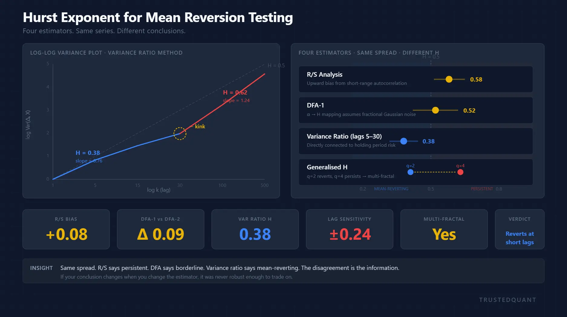
The failure mode of the variance-ratio approach is lag selection. The estimate is not constant across lag ranges. A spread might show [m]H < 0.5[/m] at short lags (say, 5 to 30 bars) and [m]H > 0.5[/m] at longer lags (100 to 500 bars), reflecting a process that reverts at short timescales but trends at longer ones. This is the estimator revealing genuine multi-scale structure in the series, and treating the resulting [m]H[/m] as a single number rather than a function of lag is where the method gets misused.

Practitioners who use the variance-ratio method need to examine the full log-log plot rather than collapsing it to a single slope estimate. A clean linear relationship across lags suggests a process with consistent scaling, and the slope is informative. A plot with a kink or a curve tells you that the Hurst exponent is scale-dependent, which is more valuable information than any single [m]H[/m] value. That kink often sits right around the holding period you were planning to trade, and ignoring it is how strategies that look mean-reverting in screening behave like random walks in production.

The Generalized Hurst Exponent Adds Flexibility at a Cost

The generalised Hurst exponent extends the analysis to arbitrary moments of the distribution by examining how [m]E[|X_{t+\tau} – X_t|^q][/m] scales with [m]\tau[/m] for different values of [m]q[/m]. At [m]q = 2[/m], this reduces to the variance-ratio approach. At [m]q = 1[/m], it uses absolute deviations. Higher values of [m]q[/m] emphasize the tails of the distribution, and varying [m]q[/m] reveals whether the scaling behavior is uniform across the return distribution or concentrated in specific quantiles.

For mean reversion testing, the generalized Hurst exponent answers a question that simpler methods cannot: whether large moves revert differently from small ones. A spread might show [m]H(q=2) < 0.5[/m] but [m]H(q=4) > 0.5[/m], indicating that typical fluctuations are mean-reverting while extreme moves are persistent. This is exactly the scenario that kills mean reversion strategies in live markets, because the strategy profits from small deviations and gives it all back on the large moves that don’t revert.

The cost of this flexibility is estimation noise. Higher-moment statistics require more data to converge, and for [m]q > 3[/m] the estimates become unreliable on the sample sizes typically available for financial spreads. A spread with two years of daily data might support stable estimates at [m]q = 1[/m] and [m]q = 2[/m] but produce effectively random results at [m]q = 4[/m]. Using these unstable higher-moment estimates to calibrate a strategy is worse than ignoring them, because they add false precision to a decision that should be made with acknowledged uncertainty.

The practical use of the generalised Hurst exponent is as a diagnostic rather than a trading signal. If [m]H(q)[/m] is approximately constant across [m]q[/m], the process is uni-fractal, and the simpler variance-ratio estimate is sufficient. If [m]H(q)[/m] varies strongly with [m]q[/m], the process is multi-fractal, the single-number Hurst exponent is misleading regardless of which method produced it, and the practitioner needs to think about whether their strategy’s exposure is concentrated in the quantiles that revert or the quantiles that persist.

Where Lag Selection Interacts With Estimator Bias

Every Hurst estimator requires a choice about scale, and this choice interacts with each method’s structural biases in ways that can reverse the conclusion about mean reversion.

The interaction runs in the same direction for R/S and DFA: including shorter blocks or windows inflates the estimate by letting short-range autocorrelation dominate the scaling fit, which compounds R/S’s existing upward bias and corrupts DFA’s exponent mapping. Widening the range to avoid this problem costs statistical power, because fewer non-overlapping segments are available at longer scales. The variance-ratio method is the exception. Its lag range directly selects the timescale of the estimate, which means the “bias” is actually a feature if the practitioner matches the lag range to their intended holding period. Fitting over lags 5 to 30 gives the Hurst exponent at the horizon where you plan to trade. Fitting over lags 5 to 500 gives an average across horizons that may not correspond to any actual trading decision. The generalised Hurst exponent inherits whichever lag sensitivity its base case ([m]q = 2[/m]) carries and amplifies it at higher moments, because tail statistics respond more sharply to which observations fall within each lag window.

There is no universal lag selection rule that resolves these issues. The honest approach is to compute the estimator over a range of lag specifications and examine the sensitivity. If the conclusion about mean reversion changes when you shift the lag range by a factor of two, the conclusion was never robust enough to trade on. If it holds across reasonable specifications, you have something worth investigating further with out-of-sample data and economic reasoning about why the spread should revert.

What to Actually Run

Given all of this, the practical recommendation is narrower than most textbook treatments suggest.

Start with the variance-ratio method, because its output connects directly to trade sizing and holding period analysis. Examine the full log-log plot rather than collapsing it to a single slope. Focus the slope estimate on the lag range that corresponds to your intended holding period. If the plot is linear across that range and the slope is clearly below 1, you have a candidate for mean reversion at the timescale you plan to trade.

Run R/S as a consistency check, not as a primary estimator. If R/S shows [m]H < 0.5[/m] despite its upward bias, the mean reversion signal is strong. If R/S shows [m]H > 0.5[/m] while the variance-ratio estimate says the opposite, investigate rather than average. The disagreement is information about the dependence structure.

Use DFA only if you have reason to believe your spread contains deterministic trends or other non-stationarities that would corrupt the variance-ratio estimate. If you do use DFA, report the polynomial order and window range, and compare DFA-1 with DFA-2 to assess sensitivity to the detrending choice.

Reserve the generalised Hurst exponent for diagnostic work on strategies that are already promising. If [m]H(q)[/m] is flat across [m]q[/m], your simpler estimates are fine. If it varies, you need to understand whether your strategy’s P&L profile is concentrated in the reverting quantiles or the persistent ones.

None of these estimators can tell you whether a spread is mean-reverting enough to trade. They can tell you whether the statistical signature of mean reversion is present at a given timescale, which is a necessary condition but not a sufficient one. The sufficient condition requires economic reasoning about why the mean exists, stress testing against execution costs, and out-of-sample validation. The Hurst exponent, properly estimated, is the first filter, and the gap between that filter and a tradeable strategy is where most of the real work remains.