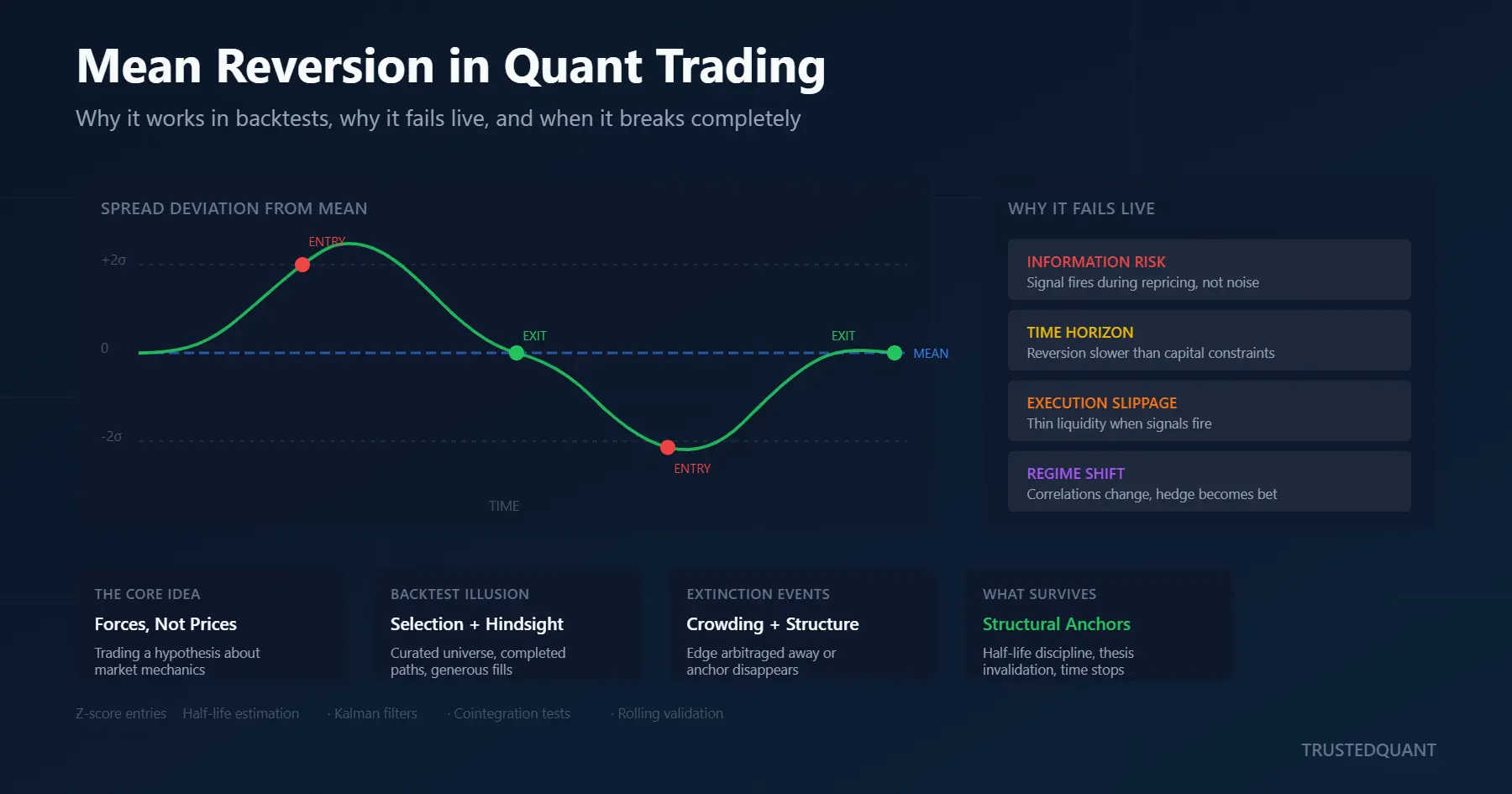
Mean Reversion in Quant Trading

Mean reversion is one of the first ideas most quantitative traders encounter and one of the last they fully understand. It feels intuitive, mathematically tidy, and easy to validate with historical data, since prices often wander away from some reference level and eventually return. That intuition is reinforced by decades of academic work, giving the impression that mean reversion reflects a deep equilibrium embedded in markets.

The danger lies not in that intuition itself, but in what it leaves out. Most losses attributed to mean reversion come not from misunderstanding the signal, but from misunderstanding the conditions under which the signal remains tradeable. The gap between a convincing backtest and a viable live strategy is structural, and no amount of parameter tuning can close it.

This page anchors the rest of TrustedQuant’s work on mean reversion. It does not attempt to teach a complete strategy or optimize parameters. Instead, its purpose is to explain what mean reversion actually represents in live markets, why it performs so well in simulation, why it fails predictably in production, and how practitioners who survive approach its implementation in Python.

What Mean Reversion Is in Practice

In practice, mean reversion is not a claim about prices returning to an average, but an assumption about underlying forces. A deviation is interpreted as a temporary imbalance, and the trade rests on the belief that mechanisms exist which tend to reduce that imbalance over time. Those mechanisms might include inventory pressure, arbitrage constraints, structural bounds, or behavioral responses. The observed price series is only the surface expression of these forces.

Because the forces matter more than the prices themselves, the object being traded is rarely a raw price. Practitioners instead construct spreads, residuals, or transformed series designed to isolate a specific relationship: equity pairs, ETF baskets, futures curves, or cash-versus-derivative positions. The “mean” being targeted is therefore a reference level implied by structure rather than a philosophical average, which is why it can shift or disappear when that structure changes.

This distinction matters because reversion is not guaranteed by mathematics alone. A series can appear stationary in historical data while being driven by relationships that no longer exert force. When the economic reason for convergence disappears, the statistical signature can linger just long enough to mislead a backtest.

For this reason, practitioners treat mean reversion as a hypothesis about market mechanics rather than a proven edge. Statistical tests can evaluate whether the hypothesis appears plausible, but they cannot justify it on their own. The gap between statistical appearance and economic reality is precisely where many backtests go wrong.

Why Mean Reversion Looks So Good in Backtests

If mean reversion is only a hypothesis, the obvious question is why it looks so compelling in backtests. The answer is that backtests benefit from structural advantages that quietly compound.

Selection narrows the universe before analysis even begins. Researchers tend to examine series that already exhibit bounded behavior, whether through explicit filters or implicit intuition. Candidates that cooperate are studied. Candidates that would have failed never enter the sample. By the time a backtest is run, the universe has already been curated toward success.

That curated universe then benefits from parameter forgiveness. Entry thresholds, lookback windows, and exit rules often have wide plateaus of acceptable performance. Small changes rarely destroy the equity curve in-sample, which makes the strategy appear stable even when many parameter combinations are simply fitting the same historical noise. Robustness checks pass because the parameters are forgiving, not because the edge is real.

The backtest also enjoys an informational advantage the live trader never has. It observes completed paths in which both the deviation and the reversion are visible. At the moment of entry, only the deviation was observable. This timing asymmetry inflates confidence in trades that carried genuine uncertainty at the time they were placed.

Execution assumptions add another layer of distortion. Mid-price fills, constant slippage, and full liquidity at signal time each appear reasonable in isolation, but together they bias results upward. The cumulative effect is an equity curve that looks stable, scalable, and repeatable, an impression that rarely survives first contact with live order books.

Why Mean Reversion Fails Live

The transition from backtest to live trading exposes mean reversion to forces that simulation systematically underweights.

Information risk is the most common failure mode. Signals often fire during periods of stress, when prices move because new information is being incorporated unevenly across instruments. The model interprets these moves as excess deviation, but the market is repricing itself. What looks like a reversion opportunity can turn out to be a trade against informed flow, causing the spread to keep widening precisely because it should.

Even when the spread eventually stabilizes, time has already done its damage. Mean reversion strategies implicitly assume that convergence occurs within a horizon compatible with capital constraints. When reversion is slow, exposure to unrelated events accumulates. The spread may still converge in the long run, but once risk limits exist, the path matters more than the destination. A strategy that is right eventually can still be bankrupt along the way.

Execution makes this problem worse. Signals often appear when liquidity is thin or one-sided, so orders placed against aggressive flow experience slippage that erodes already modest expected returns. A strategy that shows forty basis points per trade in backtest may deliver fifteen in production, which frequently falls below the threshold of viability.

Regime shifts complete the erosion. Mean reversion performs best in environments with stable correlations and bounded volatility. When those conditions change, the strategy often continues trading until losses force it to stop. Because the decay is gradual rather than dramatic, intervention is delayed and drawdowns deepen. By the time performance degradation is statistically obvious, much of the capital is already gone.

These failure modes describe degradation under stress, and degradation is often survivable. What follows is not.

When Mean Reversion Breaks Completely

While many strategies fail slowly, there are situations in which mean reversion stops working entirely, and these events often build on one another.

Crowding is the most common extinction mechanism. When enough capital trades the same relationship, the act of trading itself compresses the spread before entry and delays convergence afterward. Returns decline not because the signal has weakened, but because too many participants have noticed it. Once a relationship becomes consensus, it rarely recovers its original edge. The spread may still exist, but the profit has already been arbitraged away.

Even after crowding reduces opportunity, structural disappearance can quietly erase what remains. Statistical signatures often persist long after the underlying economic reason has vanished. Pairs that reverted because of index membership, ETF creation mechanics, or regulatory arbitrage can lose their anchor overnight following a policy change, delisting, or fund closure. Strategies that fail to monitor these assumptions end up trading relationships that no longer exist.

As these structural weaknesses accumulate, correlation breakdown can turn a hedged position into a disguised directional bet. Mean reversion implicitly assumes that hedge legs offset directional exposure. When correlations shift, the spread begins to behave like a directional trade, and losses arrive from directions the model never anticipated. At that point, the position is no longer the trade that was intended, and the risk framework no longer applies.

Recognizing these extinction events, and understanding how they cascade, is what separates strategies that degrade gracefully from those that blow up.

How Practitioners Implement Mean Reversion in Python

Surviving strategies begin with spread construction, because everything downstream depends on isolating a stable relationship. Mean reversion is not traded on raw prices but on relationships implied by structure. When that structure is misidentified, no amount of signal tuning can rescue the strategy.

This is because the raw price difference between two assets is rarely stationary. Practitioners therefore estimate hedge ratios from historical data, most commonly using ordinary least squares regression. Because these relationships drift over time, some implementations adapt the hedge ratio using rolling windows or Kalman filters. Each approach introduces tradeoffs between responsiveness, estimation noise, and lag, and the choice depends on how stable the underlying relationship is and how much error the strategy can tolerate.

With the hedge ratio established, entry logic typically relies on z-scores or Bollinger-style bands around the spread’s rolling mean. A z-score of two indicates that the spread has moved two standard deviations from its recent average, historically suggesting reversion. Practitioners avoid entering at the first threshold breach because early signals often coincide with sustained divergences. Waiting for momentum exhaustion, confirmed by a turn in the spread’s short-term direction, helps align entries with higher-probability reversions.

Holding period expectations are shaped by half-life estimation. The Ornstein-Uhlenbeck framework provides a way to estimate how quickly a spread reverts to its mean. Trades held well beyond the estimated half-life are treated as thesis failures rather than tests of patience. Time-based stops enforce this discipline by exiting positions that have overstayed their welcome regardless of where the spread stands.

Although entries attract attention, exits determine survival. A spread that continues to widen after entry may still be reverting slowly, or it may have broken entirely. Practitioners define invalidation thresholds in advance, exiting positions if the spread exceeds a defined multiple of its historical range or if the cointegration relationship fails a rolling test. Waiting for convergence after structural breakdown is how mean reversion strategies die.

Python supports this entire workflow. Statsmodels provides regression and cointegration tools, while Pykalman or FilterPy handle Kalman filter implementations. Production systems log each trade’s entry z-score, estimated half-life, actual holding period, and exit reason. Post-trade analysis compares realized behavior with model expectations, and when the two diverge consistently, the model, not the market, is assumed to be wrong. Trading stops until the discrepancy is understood.

---

For a detailed breakdown of the structural gap between simulation and production, see Why Mean Reversion Strategies Fail in Live Markets.