
Why Mean Reversion Strategies Don’t Survive Live Markets
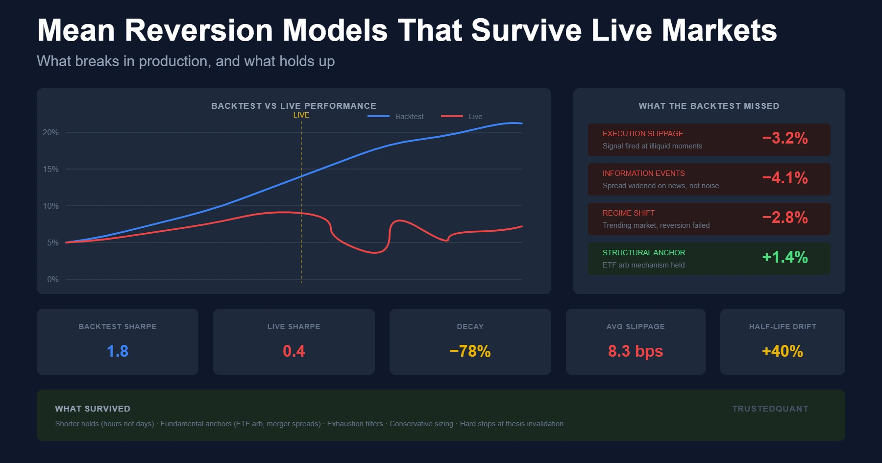
Mean reversion is easy to backtest and hard to trade. The strategy has an almost perfect record of looking good in simulation and then bleeding out once live because the failures follow predictable patterns that the backtest cannot see. The models that survive tend to share structural features that only become obvious after you understand why the others fail.
Most research in this space starts from price series that look stationary in retrospect. The spread widened and then it closed. Observing this after the fact tells you nothing about whether you could have identified the reversion before it happened or whether you could have captured it given your execution constraints and capital limits. The gap between backtest and production comes down to what the strategy is actually doing when it fires a signal.
Why Most Mean Reversion Dies
The core problem is that mean reversion signals fire precisely when something is going wrong. You buy weakness and sell strength, and the backtest assumes the weakness was temporary. In production you discover that some weakness is structural and the position keeps moving against you until your risk limits force you out.
Pairs trading on correlated equities is the canonical example. The spread between two names widens, your model fires a convergence signal, you put on the trade, and the spread keeps widening because one of the names is about to announce an accounting restatement or lose a major contract or get downgraded by three analysts in the same week. Your model saw a statistical anomaly while the market was pricing information you didn’t have.
No parameter choice fixes this. The strategy collects small gains as prices oscillate around fair value during quiet periods and gets run over when something material happens.
What Survives
Shorter holding periods reduce exposure to information events because a strategy that holds for hours is less likely to be caught by overnight news than one that holds for days. The tradeoff is that shorter horizons require better execution and more precise timing since you trade the same edge more frequently with smaller expected profit per trade.
Half-life estimation gives you a rough sense of how quickly the spread reverts.
def compute_half_life(spread_series):
    lagged = spread_series.shift(1).dropna()
    delta = spread_series.diff().dropna()
    regression = OLS(delta, lagged).fit()
    return -np.log(2) / regression.params[0]
Strategies calibrated to hold significantly longer than the estimated half-life take uncompensated risk because the spread may revert eventually but you remain exposed to everything that can happen in the meantime.
Fundamental anchors matter more than statistical relationships. A spread driven by a temporary supply-demand imbalance has a reason to close, while a spread that exists because your cointegration test found a spurious relationship has no structural force pushing it back together. The ADF test doesn’t know why two series moved together historically.
Convertible arbitrage has the bond floor and ETF stat arb relies on the creation-redemption mechanism to bound divergence, while merger arb trades against explicit deal terms that define the payout. These structural features don’t guarantee the trade works, but they provide a reason to expect convergence beyond historical correlation.
Entry Timing
Firing on the first z-score breach is almost always wrong because your backtest marks the entry at the breach level and shows the subsequent reversion, but in production the spread continues to widen for another day as the move that triggered your signal finishes playing out.
Waiting for momentum exhaustion before entering improves results in most regimes. This can be as simple as requiring the spread to stop making new extremes for some lookback window or as complex as modeling the arrival rate of directional flow. The exhaustion filter misses some reversions that happen immediately after the breach, but it avoids more of the trades that keep going against you, and the tradeoff usually favors patience.
Position Sizing and Stops
These strategies have a natural temptation to add to losers. The spread widened more so the expected profit increased so you should increase size. This logic holds if your model is right about the eventual reversion and you have unlimited capital and no risk constraints.
In practice you have a drawdown limit and a risk manager who will cut your position at the worst possible moment, so fixed fractional sizing with hard stops survives better than martingale approaches.
The stop should be based on a spread level that would invalidate the thesis rather than on a dollar loss amount, which means finding the spread level where convergence is no longer plausible and using that as your exit. Scaling into the position as the spread widens is reasonable if the total position stays within risk limits, but doubling down without a ceiling is how you produce catastrophic losses.
Regime Conditioning
Ranging markets favor mean reversion and trending markets kill it. This is obvious in retrospect and hard to identify in real time because most regime filters lag the actual regime change by enough that they don’t help much.
Volatility conditioning is more useful than trend detection. High volatility brings larger dislocations that often do revert, but the moves against you are faster and more violent as correlations spike, while lower volatility shrinks opportunities but makes behavior more predictable.
Calibrating position size and entry thresholds to the volatility regime captures some of this dynamic. Tightening entry thresholds when volatility compresses and loosening them when it expands keeps the strategy engaged across environments without taking outsize risk when conditions are unstable.
Execution Realities
These signals often fire at moments of poor liquidity because the spread widened when someone needed to move size and pushed one leg. You try to enter against that flow, and the price you saw when the signal fired may not be available once your order reaches the exchange.
Limit orders at the signal price frequently don’t fill, and market orders fill with slippage that erodes the expected profit. The edge in this strategy class is often small enough that execution costs determine whether you are profitable, so the production version of any model needs to account for this reality.
Simulating with market orders and conservative slippage assumptions is more realistic than assuming limit order fills, and if the strategy doesn’t work with 5 basis points of slippage per leg it probably doesn’t work. Even with strong structural anchors, ignoring execution realities can erase the edge.
Validation
Standard walk-forward testing misses the main failure mode because regime sensitivity doesn’t show up when optimizing on 2012-2019 since the entire period was favorable to the strategy class. Running it through 2020 or 2022 reveals what happens when the regime shifts.
The useful validation is adversarial. Find periods where the strategy class failed broadly and test there. Hostile periods include March 2020 and the 2015-2016 factor rotation and the quant quake of August 2007 and any period with sustained directional flow in your target universe. If your specific model survived those periods you need to understand why, and if it didn’t you need to understand the loss profile and decide whether you can tolerate it.
What Actually Works
The strategies that run for years without blowing up share common characteristics. Parameter count stays low with logic transparent enough that you can explain why the trade should work without referencing a cointegration coefficient. Some structural mechanism forces convergence beyond historical correlation, whether that is a bond floor or a creation-redemption process or deal terms that bound how far the spread can widen.
Sizing is calibrated to survive the worst historical drawdown with room to spare because optimizing for backtest Sharpe ensures the live drawdown will be worse than anything you tested.
The final characteristic is recognition of when to step aside. This strategy class makes money in most conditions and loses badly in specific conditions, and identifying those conditions early enough to act is the difference between a durable strategy and a blowup.
This content is for educational purposes only.
Spread the word:
