
Why Backtests Break in Live Trading
Every strategy that looked fine in simulation and then bled money live failed for reasons that were visible before capital went out. The patterns repeat because most research stacks are optimized to produce smooth equity curves, not to expose the structural leaks that appear the moment the system interacts with an exchange.
Those leaks amount to a form of overfitting that lives in execution assumptions rather than parameter selection, and the damage is just as severe. The strategy was fit to a frictionless world that never existed, where the backtest assumed prices, timing, and fills that production would never deliver.
The mismatches are mechanical. You get a fill price the market wouldn’t have given you at size, assume a latency the backtest didn’t model, and end up with a partial fill and a stub position you never planned to manage. Individually, each is small, but stacked across thousands of trades, they transform the strategy into something different from what you tested.
The backtest and the live system share code, share parameters, share intent, and remain fundamentally different objects. Understanding where they diverge is the actual work of validation, and the most common divergence starts with liquidity.
The Liquidity Lie
Backtests fill at prices that existed, an assumption that holds only while size is irrelevant. Once your order depends on available depth rather than a single historical print, the backtest stops describing an attainable outcome.
You wanted a bid that was 200 shares deep, and you needed 5,000. Historical prints don’t tell you who was leaning, who was pulling, or how quickly the book vanished when someone swept the level. Simulation engines treat past prices as if liquidity were infinite and your orders had no footprint, fitting the strategy to an execution environment that only exists in hindsight. These assumptions have real consequences in practice.
Consider a momentum strategy in mid-cap equities with an average daily volume of 500,000 shares, trading 10,000-share positions. That represents a participation rate of 2%, which seems modest. The backtest assumes you capture the closing price, but in reality, your order may move the market before it fills. The price you receive reflects how the market absorbs the information that someone wants to buy 10,000 shares. In liquid names during calm periods, the cost might be a few basis points. In thinner names or stressed conditions, it can spike dramatically.
The asymmetry intensifies when the signal fires during movement. Momentum attracts flow, and other participants who noticed the same price change are competing for the same liquidity while liquidity providers retreat, leaving the book thinner than usual. Your 2% participation rate calculated on average volume can quickly become 8% of the available liquidity at that moment. Even a simple model that accounts for book depth, volatility, participation, and concurrent flow produces a much lower realized return than the naive backtest.
This is precisely the point. The gap between assuming you get the closing price and modeling even a crude version of market impact is where backtests mislead you. Liquidity determines the price you capture; execution topology determines when and whether your order fills at all. Both dimensions interact, compounding small divergences across thousands of trades into measurable P&L drag.
Execution Topology
Execution adds another layer of divergence between backtest and reality. Backtests treat the path from signal to fill as instantaneous, but production never behaves that way.
Imagine your signal fires at 10:02:34.127. Computing it across 500 names takes 340 milliseconds. The order management system then receives the signal, applies risk checks, and queues the order over another 50 milliseconds. Your broker’s smart order router spends 80 milliseconds selecting venues before sending the order to the exchange, where it enters the matching engine queue. Total latency from signal to acknowledgment runs 600 milliseconds on a good day and stretches to two seconds under stress.
During that delay, prices move and liquidity shifts. The fill you modeled may no longer exist. Partial fills illustrate the cost clearly. A backtest assumes you bought 5,000 shares, but production fills only 2,300 before the price moves away. You now hold a position that is too small to matter and too large to ignore. Decisions multiply: do you chase the remaining shares at worse prices or cancel and hold the stub? Your actual P&L is determined by managing this incomplete position, a scenario the backtest never anticipated.
Queue position affects mean reversion strategies in the same way. A technical level might appear filled in historical data, but in reality, sitting deeper in the queue means the selling pressure continues. You receive the fill on the way down, missing the bounce entirely.
None of these are edge cases. Run any systematic strategy for a month and you’ll accumulate hundreds of instances where the backtest’s execution model diverged from what actually happened, each divergence small on its own, compounding into significant P&L drag.
Execution latency costs basis points, but the decay of your signal costs alpha itself. Delays in capturing the move, compounded by other participants acting on the same information, shrink the realized return relative to the backtest. This pattern is predictable enough to simulate but invisible without careful measurement.
Signal Decay and Alpha Half-Life
In a backtest, historical data gets replayed as if your signal existed in isolation, but in reality, it never does. Every price move you observe already carries the footprint of other participants acting on the same or correlated information. Deploying capital places you inside that flow instead of outside it, and the alpha you thought persisted for two days often collapses to two hours once multiple players compete to capture the same move. Observing this in production reveals just how fleeting some edges can be.
The pace at which alpha decays shapes both position sizing and execution urgency. Track the interval between signal generation and fill, and you see how much of the theoretical alpha survives in practice.
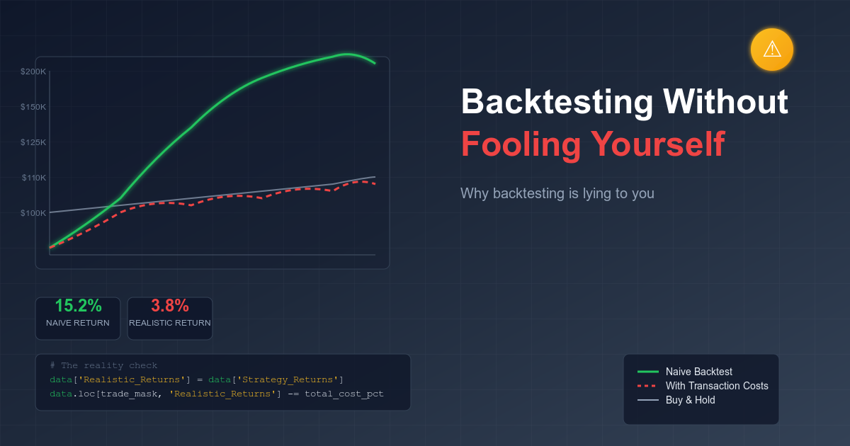
A strategy that shows 15% annualized on daily bars assumes you capture the full daily move, but factoring in realistic execution delays and partial fills typically reduces that capture to 60%. When limit orders are filled precisely as the market moves against you, the realized alpha can drop further to 40%. What looked like 15% on paper may shrink to 6%, barely clearing transaction costs, and each trade exposes the fragility of the assumed edge.
The problem is magnified when signals are widely replicated. Momentum based on price and volume is visible to nearly everyone in the market, which shortens the alpha’s half-life. Proprietary datasets or unusual transformations decay more slowly, offering a longer window to act. Backtests cannot measure this decay directly, but by examining captured alpha against execution delays, the pattern emerges. The insight informs not just whether the signal is valid but how quickly it must be executed.
Modeling this decay in a backtest requires more than generic slippage. You need to incorporate partial fills, latency, and adverse selection in a way that mirrors production conditions. Plotting captured alpha against delay across trades exposes where the edge is real and where it evaporates. This approach turns a backtest from a simple performance estimate into a diagnostic tool, guiding both signal design and execution strategy while revealing how fragile an apparent advantage can be once it enters the market.
Reconciliation as Validation
Watching a strategy in motion exposes what a backtest can never fully reveal. Paper trading puts orders into real markets without committing capital, and in those moments, timing drifts, partial fills, and queue position effects quickly become apparent. You see the assumptions about fills and execution unravel in ways a smooth equity curve never warned you about.
Even observing these mechanics is only the beginning. Paper trading cannot uncover capacity constraints or the impact of crowded trades because your orders are too small to move markets. A few weeks of simulated execution cannot reveal failures that appear only in specific market regimes. To understand where a strategy truly breaks, reconciliation must extend over months, accumulating evidence that highlights persistent patterns and structural weaknesses.
The work begins with trade-level comparison. Start with a structured comparison of every trade. For each one, match backtest assumed price against live fill price, assumed time against fill time, and target shares against filled shares. Flag discrepancies above a threshold and run the comparison daily. The patterns that emerge matter more than the averages.
def reconcile(backtest, live, slippage_bps=5):
    breaks = []
    for bt, lv in zip(backtest, live):
        price_gap = abs(lv.price - bt.price) / bt.price * 1e4
        time_gap = (lv.time - bt.time).total_seconds()
        fill_ratio = lv.size / bt.size

        if price_gap > slippage_bps or time_gap > 1 or fill_ratio < 0.95:
            breaks.append((bt.symbol, price_gap, time_gap, fill_ratio, lv.time.hour))
    return breaks
Run daily and aggregated over time, the output stops looking like noise. Slippage clustering at market open points to execution timing assumptions that don’t hold for that period. Certain names slipping more than expected means your liquidity model is miscalibrated for that segment of the universe. If timing drift has increased over the past month, the signal is probably getting more crowded, and fill rates below 90% on momentum signals reveal that the book is thinner than you assumed when the signal fires.
Each pattern points to a specific fix, which is what makes reconciliation valuable. Average slippage of 8 basis points sounds trivial, but 15 basis points concentrated in small-cap names during the first hour identifies exactly where alpha is leaking. Observing these deviations trade by trade uncovers the slow erosion of performance that backtests disguise.
The work is tedious, the process unglamorous, and it does not produce elegant research papers or smooth backtest curves, yet the actual alpha leakage happens here, trade by trade, and the only way to stop the leak is to measure it with enough granularity to diagnose the cause.
What Validation Actually Looks Like
Validation isn’t a gate you pass before going live but an ongoing process of measuring the gap between backtest and reality while working to understand why it exists.
The strategies that survive share a common trait, though not the one you might expect. The team understood the backtest’s limitations before deployment, built monitoring to detect when those limitations bind, and had a plan for what to do when they did. Whether a strategy captures something real is decided upstream, and validation tells you whether your implementation preserved it.
By the same logic, backtests make assumptions; production exposes which ones survive contact with the market, and reconciliation shows where they stop holding. Without all three, you’re hoping rather than validating.
A backtest that only survives at 10 basis points of assumed slippage reveals that the execution assumption is doing the heavy lifting. Once you model execution correctly, accounting for realistic delays, partial fills, adverse selection, and crowding, the alpha often isn’t there. Better to discover this through reconciliation analysis than through a conversation with your risk committee.
Careful validation gives you a map of the specific ways the strategy will break along with a monitoring system that watches those fault lines in production.
This content is for educational purposes only.
Spread the word:
