
Overfitting a Backtest: How to Measure It and What It Costs You
Somewhere between the third and thirtieth parameter sweep, every systematic trader crosses an invisible line. The strategy starts fitting signal, then it starts fitting noise, and the backtest cannot tell you which transition happened when. The equity curve just keeps improving. By the time you select your “optimal” configuration and move to out-of-sample testing, the damage is already embedded in your process, and the standard defences against it are far weaker than most practitioners realise.
The usual advice (simplify the model, hold out data, run walk-forward analysis) treats overfitting as a modelling error that careful hygiene can prevent. What Bailey, López de Prado, and colleagues showed across a series of papers between 2012 and 2015 is that overfitting in backtesting is fundamentally a multiple testing problem, one that holdout methods do not and cannot solve because they ignore the variable that matters most: the number of trials you ran before selecting your strategy. Without controlling for that count, out-of-sample testing is a second roll of the same loaded dice.
What follows builds a deliberately overfit strategy from scratch, applies the standard defences, shows exactly how and why they fail, and then introduces the correction that actually works.
Building the Overfit
Consider a simple monthly trading strategy applied to a synthetic random walk. The strategy has four parameters: entry day (which business day of the month to enter), holding period (how many days to hold), stop loss (a threshold multiple of volatility that triggers an early exit), and side (long or short). Even with these minimal degrees of freedom, the combinatorial space is large enough to guarantee finding a configuration that looks profitable on any finite sample of random data.
import numpy as np
import pandas as pd

np.random.seed(42)
T = 1000
returns = np.random.normal(0, 0.01, T)
prices = 100 * np.cumprod(1 + returns)

best_sr, best_params = -np.inf, None
for entry_day in range(1, 23):
    for hold in range(1, 21):
        for stop in range(1, 11):
            for side in [1, -1]:
                pnl = []
                i = 0
                while i < T:
                    if (i % 22) + 1 == entry_day:
                        entry_price = prices[i]
                        for d in range(1, hold + 1):
                            if i + d >= T:
                                break
                            ret = side * (prices[i + d] / entry_price - 1)
                            if ret < -stop * 0.01:
                                pnl.append(-stop * 0.01)
                                break
                        else:
                            if i + hold < T:
                                pnl.append(side * (prices[i + hold] / entry_price - 1))
                        i += hold
                    else:
                        i += 1
                if len(pnl) > 10:
                    sr = np.mean(pnl) / np.std(pnl) * np.sqrt(12)
                    if sr > best_sr:
                        best_sr, best_params = sr, (entry_day, hold, stop, side)

print(f"Best IS Sharpe: {best_sr:.2f}, Params: {best_params}")
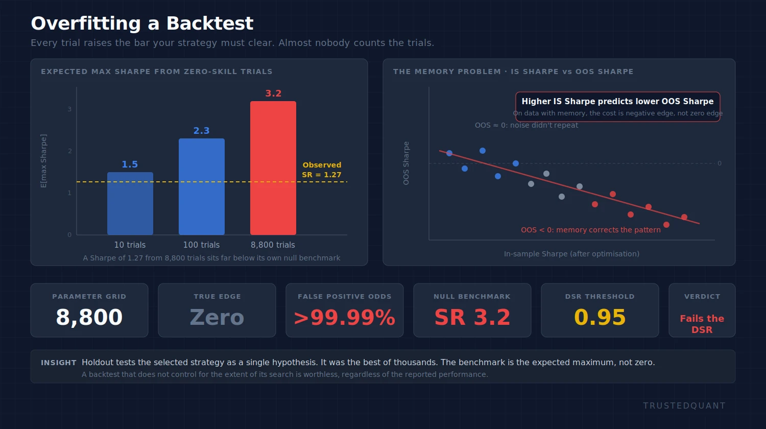
The search explores 22 × 20 × 10 × 2 = 8,800 parameter combinations, and on most seeds it finds an annualised Sharpe ratio above 1.0 in-sample. This result is entirely manufactured: the underlying series is a random walk with zero drift, so no profitable strategy can exist by construction. The elevated Sharpe ratio is a pure artefact of selection, the consequence of picking the single best outcome from thousands of trials and treating it as if it were the only trial that occurred.
This is the core mechanic of backtest overfitting, and it operates identically whether the strategy is simple or complex, hand-coded or machine-learned. The number of parameter combinations explored determines the probability that at least one configuration will appear statistically significant by chance. For 8,800 independent trials at a 5% significance level, the probability of finding at least one false positive exceeds 99.99%.
The Holdout Defence
The standard response is to split the data. Train on the first half, test on the second half, and only trust strategies that perform well out of sample. This is the holdout method, and it is the single most widely recommended defence against overfitting in both academic and practitioner literature.
prices_is = prices[:T // 2]
prices_oos = prices[T // 2:]

def run_strategy(p, params):
    entry_day, hold, stop, side = params
    pnl = []
    i = 0
    while i < len(p):
        if (i % 22) + 1 == entry_day:
            entry_price = p[i]
            for d in range(1, hold + 1):
                if i + d >= len(p):
                    break
                ret = side * (p[i + d] / entry_price - 1)
                if ret < -stop * 0.01:
                    pnl.append(-stop * 0.01)
                    break
            else:
                if i + hold < len(p):
                    pnl.append(side * (p[i + hold] / entry_price - 1))
            i += hold
        else:
            i += 1
    if len(pnl) > 5:
        return np.mean(pnl) / np.std(pnl) * np.sqrt(12)
    return 0.0

best_sr_is, best_params_is = -np.inf, None
for entry_day in range(1, 23):
    for hold in range(1, 21):
        for stop in range(1, 11):
            for side in [1, -1]:
                sr = run_strategy(prices_is, (entry_day, hold, stop, side))
                if sr > best_sr_is:
                    best_sr_is = sr
                    best_params_is = (entry_day, hold, stop, side)

oos_sr = run_strategy(prices_oos, best_params_is)
print(f"IS Sharpe: {best_sr_is:.2f}, OOS Sharpe: {oos_sr:.2f}")
In most runs the OOS Sharpe is poor, which is what you would expect: the strategy was fit to noise in the first half, and the noise pattern did not repeat in the second half. This is the textbook case, and it makes holdout look like it works.
The problem emerges when you repeat the process. If you run the full sweep, find a strategy, test it out of sample, reject it, then try a different specification and test again, and keep going, you are now running multiple trials on the OOS dataset itself. After enough iterations you will find a strategy that performs well both in-sample and out-of-sample purely by chance, because you have turned the OOS test into a second search. The holdout did not fail because of bad luck; it failed because it does not account for the number of times it was applied.
oos_sharpes = []
for seed in range(200):
    np.random.seed(seed)
    r = np.random.normal(0, 0.01, T)
    p = 100 * np.cumprod(1 + r)
    p_is, p_oos = p[:T // 2], p[T // 2:]

    best_is, best_p = -np.inf, None
    for ed in range(1, 23):
        for h in range(1, 21):
            for s in range(1, 11):
                for sd in [1, -1]:
                    sr = run_strategy(p_is, (ed, h, s, sd))
                    if sr > best_is:
                        best_is, best_p = sr, (ed, h, s, sd)

    oos_sharpes.append(run_strategy(p_oos, best_p))

oos_sharpes = np.array(oos_sharpes)
print(f"Fraction with OOS SR > 0.5: {(oos_sharpes > 0.5).mean():.2%}")
print(f"Max OOS Sharpe across seeds: {oos_sharpes.max():.2f}")
Running this across 200 independent random walk seeds, each with its own in-sample optimisation and out-of-sample validation, produces a non-trivial fraction of seeds where the OOS Sharpe exceeds 0.5, and in some cases exceeds 1.0. If you were a researcher who happened to use one of those seeds (or equivalently, a firm that happened to develop during one of those periods), you would conclude that your strategy passed the holdout test. The critical information that would change your assessment, the fact that this was one of 200 attempts, is exactly the information that holdout does not capture and cannot incorporate.
Bailey et al. make this point formally: the holdout method “does not take into account the number of trials attempted before selecting a particular strategy configuration, and consequently holdout cannot correctly assess a backtest’s representativeness.” This is not a minor technical qualification. It is a structural limitation that makes holdout unreliable precisely in the situation where it is most needed, which is when a researcher has explored a large space of strategies before presenting the final candidate.
The Expected Maximum Sharpe Ratio
The correction starts with a simple observation: if you draw [m]N[/m] independent Sharpe ratio estimates from a distribution with mean [m]\mu[/m] and standard deviation [m]\sigma[/m], the expected maximum of that set grows with [m]N[/m]. Bailey and López de Prado derive an approximation for this expected maximum using extreme value theory:
where [m]\gamma \approx 0.5772[/m] is the Euler-Mascheroni constant, [m]\Phi^{-1}[/m] is the inverse standard normal CDF, and [m]e[/m] is Euler’s number.
from scipy.stats import norm

def expected_max_sr(n_trials, mu=0, sigma=1):
    emc = 0.5772156649
    z1 = norm.ppf(1 - 1.0 / n_trials)
    z2 = norm.ppf(1 - 1.0 / (n_trials * np.e))
    return mu + sigma * ((1 - emc) * z1 + emc * z2)

for n in [10, 100, 1000, 8800]:
    print(f"N={n:>5}: E[max SR] = {expected_max_sr(n):.2f}")
The output shows that with 8,800 independent trials (our parameter sweep), the expected maximum Sharpe ratio under the null of zero true skill is approximately 3.2. With 100 trials it is around 2.3. Even with just 10 trials, you can expect to see a Sharpe above 1.5 purely by chance. The implication is that any reported Sharpe ratio must be evaluated against this threshold, not against zero, and the threshold rises with every trial you run.
This is the piece that holdout and walk-forward analysis both miss. They evaluate the selected strategy as if it were a single hypothesis tested once, when in reality it was the best of many hypotheses tested on the same data. Adjusting for this is not optional; without it, you are comparing your result to the wrong benchmark.
The Deflated Sharpe Ratio
The Deflated Sharpe Ratio (DSR) operationalises this correction. It computes the probability that a strategy’s observed Sharpe ratio is genuinely greater than zero after adjusting for the number of trials, the variance across those trials, the sample length, and the non-normality of returns (skewness and kurtosis). The formula builds on the Probabilistic Sharpe Ratio (PSR) by replacing the zero benchmark with the expected maximum Sharpe ratio under the null:
def deflated_sharpe_ratio(sr_observed, sr_benchmark, T, skew, kurt):
    num = (sr_observed - sr_benchmark) * np.sqrt(T - 1)
    denom = np.sqrt(1 - skew * sr_observed + (kurt - 1) / 4 * sr_observed**2)
    return norm.cdf(num / denom)

sr_hat = 1.27
n_trials = 8800
T_obs = 1000
sr_bench = expected_max_sr(n_trials, mu=0, sigma=1)
dsr = deflated_sharpe_ratio(sr_hat, sr_bench, T_obs, skew=0, kurt=3)
print(f"Observed SR: {sr_hat:.2f}")
print(f"Benchmark SR (E[max]): {sr_bench:.2f}")
print(f"Deflated Sharpe Ratio: {dsr:.4f}")
A DSR below 0.95 means you cannot reject the null hypothesis that the strategy’s performance is entirely explained by selection from multiple trials, at the 5% significance level. In the example above, a Sharpe of 1.27 from 8,800 trials on 1,000 observations produces a DSR well below 0.95, which is exactly what you should expect when the underlying process is a random walk. The strategy is not merely unreliable; there is no statistical basis for believing it has any skill at all.
The DSR framework forces you to track and report something that almost no backtest publication includes: the number of trials. Without that number, there is no way to compute the appropriate benchmark, and without the benchmark, the reported Sharpe ratio is uninterpretable. Bailey and López de Prado argue that “a backtest where the researcher has not controlled for the extent of the search involved in his or her finding is worthless, regardless of how excellent the reported performance might be.” For why backtests break in live trading, the multiple testing problem is often the invisible root cause that practitioners diagnose as regime change or bad luck.
The Memory Problem
The cost of overfitting extends beyond merely producing zero expected returns out of sample. Bailey et al. prove a result with severe practical consequences: on time series with memory (autoregressive or mean-reverting processes, which describe most financial data), overfitted strategies produce negative expected returns out of sample, systematically.
The intuition runs as follows. An overfitted strategy identifies the most extreme random patterns in the in-sample data and builds trading rules to exploit them. On a memoryless process like a coin toss, those patterns simply fail to repeat, producing zero expected performance. But on a process with memory, extreme patterns are actively corrected by the autocorrelation structure. A mean-reverting series that deviated strongly in one direction during the in-sample period will tend to reverse in the out-of-sample period, and the overfitted strategy, which was built to profit from that exact deviation, now finds itself positioned on the wrong side of the correction.
This transforms the cost of overfitting from “no edge” to “negative edge.” The more severely overfit the strategy, the more extreme the in-sample patterns it captured, and the more violent the reversal it faces. Bailey et al. describe this as the strategy accumulating “memory against its future performance,” where deeper in-sample optimisation creates progressively worse out-of-sample outcomes. The relationship between in-sample and out-of-sample Sharpe ratios is not flat but negatively sloped: higher IS performance predicts lower OOS performance, a finding they demonstrate empirically using their combinatorially symmetric cross-validation (CSCV) framework.
For practitioners, this means that the standard operating procedure of optimising a strategy and then deploying the best-performing configuration is not merely ineffective on financial data but actively counterproductive. The strategy you select as optimal in-sample is, under memory, the strategy most likely to lose money going forward.
What Actually Protects You
If holdout and walk-forward analysis are insufficient, and if the expected maximum Sharpe ratio and DSR provide the diagnostic, the remaining question is what a practitioner should actually do differently.
The first and most important change is structural: track the number of trials. Every parameter combination tested, every specification explored, every in-sample optimisation run, all of it counts toward [m]N[/m] in the expected maximum formula. Most research processes do not record this number, which makes it impossible to compute the DSR after the fact. The discipline of maintaining a trial log changes the economics of exploration, because every additional test raises the bar that the final strategy must clear.
The second change involves the evaluation criterion itself. Rather than asking “does this strategy have a positive OOS Sharpe?” you should ask “does this strategy’s OOS Sharpe exceed the expected maximum Sharpe under the null, given the number of trials I ran?” The DSR encodes this question directly. A strategy with a DSR above 0.95 has a Sharpe ratio that is unlikely to have emerged from pure selection, even after accounting for the full search. A strategy with a DSR below 0.95 is indistinguishable from the best random draw.
The CSCV framework from Bailey et al. provides a third layer of protection, producing a probability of backtest overfitting (PBO) that estimates how likely it is that the IS-optimal strategy underperforms the median of all strategies OOS. Unlike holdout, CSCV generates its estimate from all possible symmetric splits of the data rather than a single arbitrary partition, making it robust to the choice of split point. A PBO above 0.05 is a strong signal that the strategy selection process has overfit.
None of these tools eliminate overfitting entirely. What they do is quantify it, transforming the question from “is this strategy overfit?” (which holdout pretends to answer with a yes/no) into “how likely is it that this strategy’s performance is explained by selection?” (which DSR and PBO answer with a probability). That probability, combined with the trial count, gives you the information you need to make an allocation decision rather than a guess.
For what distinguishes strategies that survive this scrutiny from those that do not, see what makes a strategy survive out of sample.
What It Costs You
Research teams that do not track trial counts cannot distinguish genuine discoveries from statistical artefacts, and over time the artefacts accumulate in the portfolio. Strategies that require either stronger signals or fewer trials to clear the DSR threshold get crowded out by overfit configurations that looked convincing in isolation, and the fund’s strategy roster becomes populated disproportionately by backtests that never controlled for the full extent of the search that produced them. On financial data with memory, these are not merely inert holdings producing zero returns; they are actively accumulating losses as the autocorrelation structure corrects the in-sample patterns they were built to exploit.
The cost compounds silently because the feedback loop is slow. An overfitted strategy can take months or years to demonstrate conclusive underperformance, during which time it consumes capital and displaces allocations to strategies that might have genuine edge. By the time the degradation is acknowledged, the research team has already moved on to the next round of backtesting, likely without adjusting their process, which means the next batch of strategies passes through the same uncontrolled selection filter.
Controlling for that search is not a refinement of the standard backtesting process. It is a prerequisite for the process to mean anything at all.
Spread the word:
