
Walk-Forward Optimization Isn’t Enough
Walk-forward optimization is the procedure most desks trust to keep overfitting out of a backtest. Fit the parameters on an in-sample window, score the chosen configuration on the next block the optimizer never saw, roll forward, and join the out-of-sample segments into one equity curve. No segment was optimized on, so the curve reads as an honest out-of-sample estimate. That clean rolling curve becomes the evidence that releases capital.
A gap hides inside that clean curve. Each segment is scored once, so the result is treated as a single test. Yet the analyst reaches it only after running many configurations: indicator families, parameter grids, and the settings of the walk-forward scheme itself. The count of trials behind the reported curve is large, and none of it is recorded. Bailey and López de Prado made the consequence precise. Under enough skill-less trials the expected maximum Sharpe grows without bound, and a holdout cannot correct for a trial count it never tracked. Their summary is blunt: a backtest that does not control for the extent of its search is worthless, however strong the performance looks.
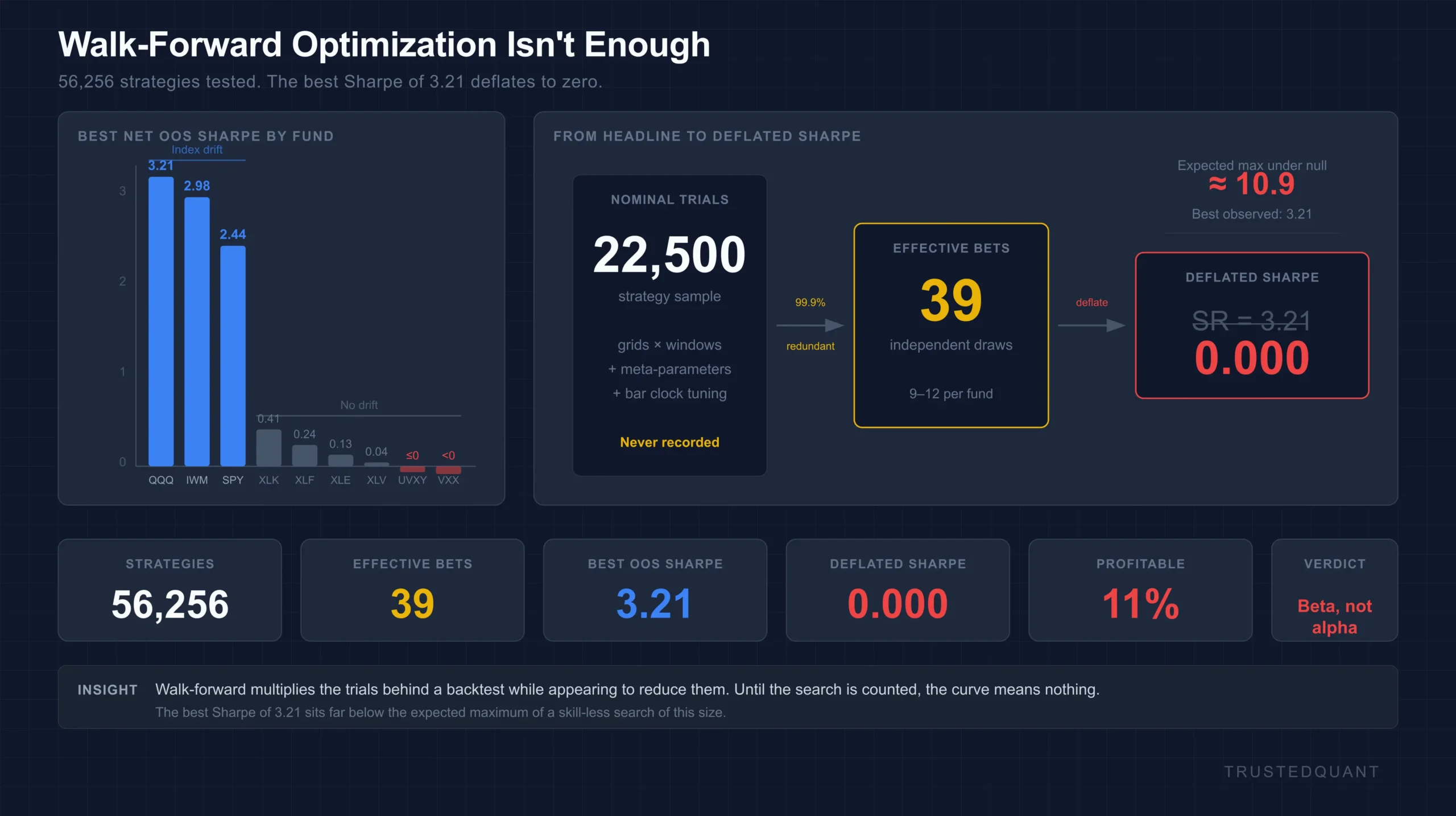
To see how wide the gap runs, execute the procedure at scale and count what it searched. What follows runs 56,256 technical-analysis strategies through rolling walk-forward on nine US equity ETFs, all realistically costed, and deflates the winner against the multiple-testing null. The headline survives none of it.
The Corpus and Its Best Sharpes
Those strategies run on one-minute US equity ETF data from 2007 to 2024, aggregated into dollar bars within regular trading hours, across nine funds: the index proxies SPY, QQQ, and IWM; the sector funds XLE, XLF, XLK, and XLV; and the volatility products UVXY and VXX. Six indicator families cross with stop and target brackets and a long-or-short switch, roughly 6,250 configurations per fund. Friction is charged per fill: a time-of-day half-spread, a commission on a realistic order notional, and short-borrow on every short leg. Signals are causal, filled at the next bar’s open, with stops and targets read off intrabar highs and lows.
Read at the level a validation memo stops at, the corpus is a success. Net out-of-sample Sharpe peaks at 3.21 on QQQ, 2.98 on IWM, and 2.44 on SPY, all after costs (Figure 1). A book built from the per-fund winners would carry index Sharpes above 2 and a smooth curve, and sizing is the natural next move. The sector and volatility funds, with no comparable drift to capture, sit at or below zero: XLK at 0.41, XLF at 0.24, XLE at 0.13, XLV at 0.04, VXX slightly negative.
That distance between the index funds and everything else is the first clue that the search found exposure rather than skill. Confirming it means counting the trials behind the 3.21.
The Trial Count You Didn’t Record
Scoring several out-of-sample blocks instead of one makes walk-forward look more rigorous than a single holdout. Each block sits at the end of its own in-sample optimization, and the scheme that produced the blocks carries choices of its own.
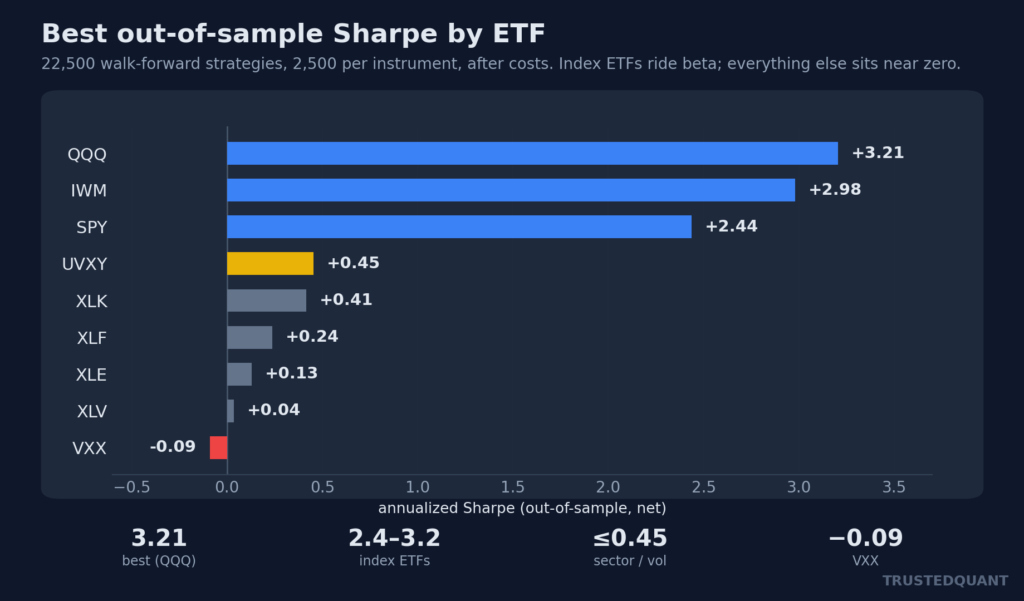
Figure 1: Best net out-of-sample Sharpe per fund. The three broad-index funds clear 2.4; the sector and volatility funds sit near or below zero.
Window length, step size, the in-sample to out-of-sample ratio, the reoptimization cadence, and the bar clock are each a degree of freedom, tuned by watching the aggregate curve and keeping whatever lifts it. The bar clock alone is open-ended once minute data sits underneath. A dollar-bar threshold is a continuous knob; sliding it changes which trades exist and where the stops fall. Retuning that clock until the curve smooths is a search in itself, run without leaving a record.
Behind the final curve sits the count of windows times the per-window grid times every meta-parameter setting that was tried and dropped, and none of it registers in the walk-forward efficiency ratio. The statistic that does begins with a fact about maxima. Draw [m]N[/m] skill-less Sharpe estimates with dispersion [m]\sigma[/m], and the expected largest of them grows with [m]N[/m]:
$$E\left[\max \widehat{SR}_N\right] \approx \sigma \left[(1 – \gamma)\,\Phi^{-1}!\left(1 – \tfrac{1}{N}\right) + \gamma\,\Phi^{-1}!\left(1 – \tfrac{1}{Ne}\right)\right].$$
At the scale of this corpus, that factor reaches about 4 at 22,500 trials. Multiplied by the dispersion of the trial Sharpes present in this corpus, near 2.7 in annualised units, the benchmark for a 22,500-trial search lands close to 10.9, well above the 3.21 the search produced. Even that figure is too generous, because most of the 22,500 strategies are not independent draws.
From 22,500 Trials to 39 Bets
Reparameterizations of one idea move together. A crossover at a 48-bar lookback and one at 50 bars produce nearly the same out-of-sample series, so counting each as a separate trial overstates how much was searched. Effective breadth is the honest count, the number of mutually independent bets inside the nominal total. The eigenvalue participation ratio of the strategy-return correlation matrix measures it: the squared sum of the eigenvalues over their sum of squares. Across the 22,500-strategy sample it comes to 39, and inside a single fund it runs between 9 and 12, so QQQ’s 2,500 strategies carry the information of about 12 independent bets (Figure 2). Nominal and effective breadth differ by one to two orders of magnitude.
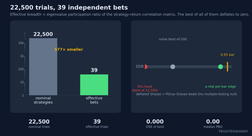
Figure 2: Nominal versus effective breadth, and the deflated Sharpe. The 22,500 strategies reduce to 39 independent bets; the best of all of them deflates to 0.000 against a real edge at 0.87 and the 0.95 bar.
With the effective count in hand, the deflation is a short calculation: it returns the same verdict whether [m]N[/m] is the nominal 22,500 or the effective 39.
Deflating the Best Survivor
The deflated Sharpe ratio turns the benchmark into a probability: whether a strategy’s observed Sharpe is genuinely above zero once the trial count, the dispersion across trials, the sample length, and the non-normality of the returns are all charged against it. It replaces the zero benchmark of the probabilistic Sharpe ratio with the expected maximum under the null.
def deflated_sharpe(sr, sr0, T, skew, kurt):
    z = (sr - sr0)*np.sqrt(T-1) / np.sqrt(1 - skew*sr + (kurt-1)/4*sr**2)
    return norm.cdf(z)

deflated_sharpe(best_sr, expected_max_sr(22500, sharpes.std()), T, g3, g4)   # 0.000
On this corpus the best strategy returns 0.000, but the routine discriminates: the same routine returns 0.87 on a constructed per-bar edge and 0.32 on the best of 200 pure-noise strategies, against a 0.95 bar. One caveat keeps it honest: the benchmark near 10.9 is inflated by the spread between QQQ above 3 and the volatility funds below zero, a dispersion of factor exposures rather than a symmetric skill-less population. That leaves the deflated Sharpe and the effective-trial count as the load-bearing numbers, since neither leans on that symmetry, and both land in the same place. Two readings of the corpus explain where the apparent alpha came from.
The Sharpe Was Beta
One reading is the shape of the full population. Across all 56,256 strategies, aggregated to daily returns, the median net Sharpe is [m]-3.2[/m] and only 11% are profitable after costs; the single best, 4.44, sits far inside the expected maximum of a skill-less search of that size, near 12, so a fully costed technical book on these funds loses money end to end. The few positive Sharpes at the right edge are what a search returns from a heavy-tailed loss distribution.
Those positive Sharpes also concentrate in one place. Seventeen years of long-side drift in SPY, QQQ, and IWM is captured by almost any long-biased parameterization, which is why thousands cluster at Sharpe 2 to 3 while the driftless sector and volatility funds sit near zero. Overfitting probability lands near zero as well, the kind of number that clears a review, because it counts how often the in-sample winner falls into the bottom half out-of-sample, and here the ranking is stable only because it tracks the same beta throughout. A near-zero overfitting probability sitting beside a zero deflated Sharpe is the signature of mined factor drift.
Beta could be blamed for the index result, so the cleanest check strips it out. One dual moving-average crossover, optimized over 136 lookbacks per fund on the same costed bars, gives a best in-sample Sharpe of 0.31 against an expected maximum of 0.44, already below its own null. It deflates to 0.32, and the 136 grid points reduce to about 3 independent bets, so the same mechanism holds inside one family where the only thing left to blame is selection.
What Walk-Forward Protects and Leaves Exposed
None of this convicts walk-forward as a procedure. A single pre-committed run, one configuration fixed before anyone looks at the data, returns a genuinely unbiased out-of-sample estimate, though it is noisy: the aggregate out-of-sample Sharpe of a zero-edge configuration has a standard deviation near 0.5 over a few years, which follows from the sampling distribution of a Sharpe estimate. Many skill-less configurations therefore clear any fixed threshold by luck. The procedure is sound; almost nobody runs it once.
What restores the meaning is recording the search. Every parameter combination, specification, in-sample optimization, and meta-parameter of the scheme counts toward [m]N[/m], and a corpus that never logged [m]N[/m] cannot be deflated after the fact. The effective number of trials, the deflated Sharpe, and the probability of backtest overfitting belong next to the equity curve, not in an appendix. Skipping them is expensive in a way that is slow to show: on financial data with memory, the in-sample patterns an overfit configuration was built to exploit tend to reverse out of sample, so the curves that looked best going in are the ones most likely to lose going forward.
Walk-forward optimization multiplies the trials behind a backtest while appearing to reduce them, because each out-of-sample segment is counted as a single evaluation and the search that selected the configuration is never written down. Until that search is counted, the out-of-sample curve means nothing.
For the apparatus behind the deflated Sharpe, see Overfitting a Backtest; for what separates the strategies that survive it, see What Makes a Strategy Survive Out of Sample.
This content is for educational purposes only.
Spread the word:
