
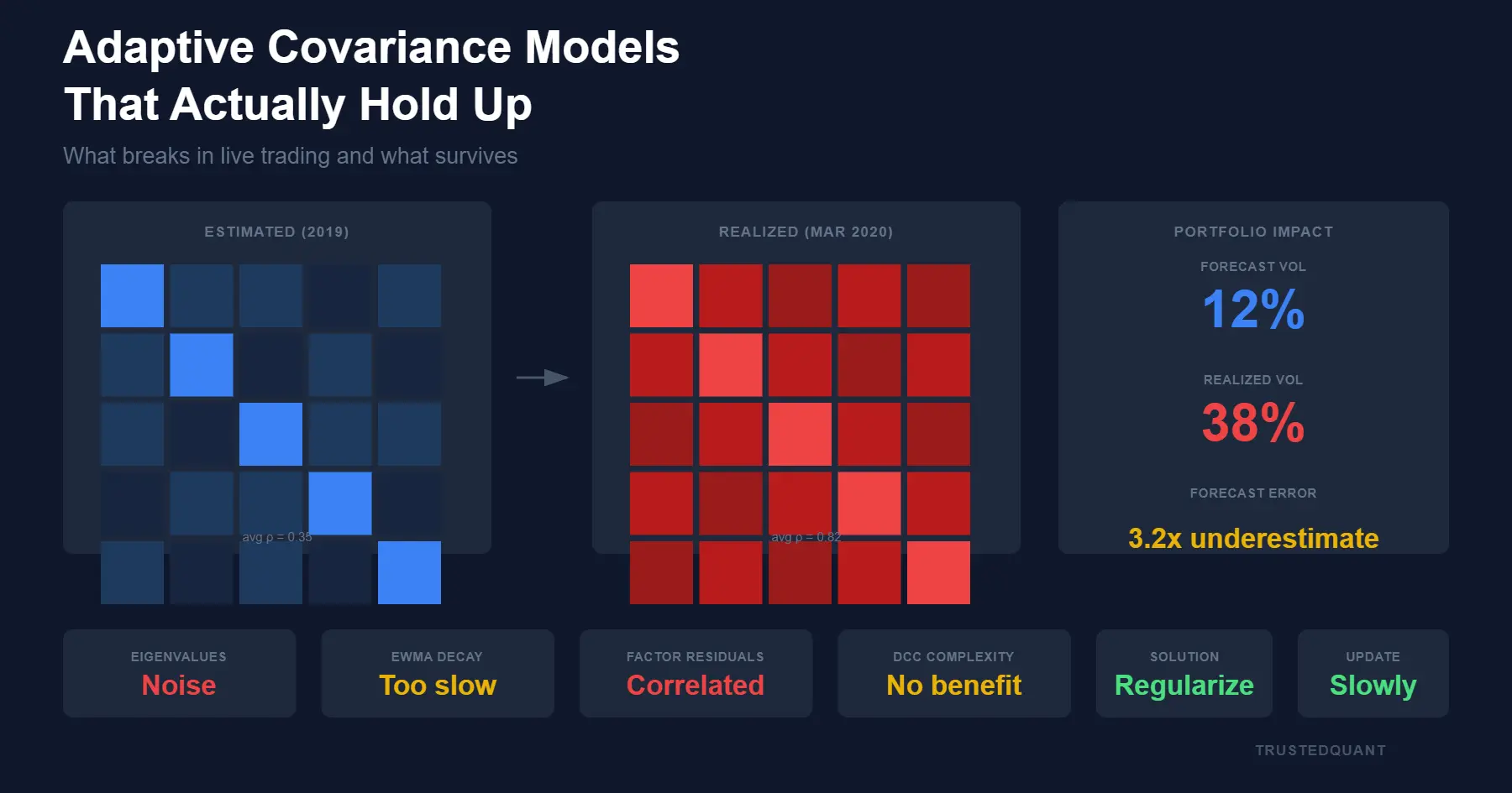
Adaptive Covariance Models That Actually Hold Up in Live Trading
Sample covariance from a rolling window will blow up your portfolio. Shrinkage, factor decomposition, or exponential weighting can help, but letting the model adapt continuously to incoming data often fails just as badly. This pattern repeats across firms and decades, with backtests looking promising, live performance degrading within months, and risk limits breached during the first correlation spike.
Why Adaptive Models Fail Fast
Backtest covariance is stale by construction because you estimate relationships that existed rather than relationships that will exist. The appeal of adaptive models follows directly from this staleness since letting estimates track the market seems like the obvious fix. DCC-GARCH updates correlation dynamics daily based on standardized residuals, and it looks elegant on paper.
Correlation spike clustering breaks that logic. When volatility expands correlations rise, and when correlations rise in your estimator portfolio weights shift toward assets that appear diversifying. Those assets are diversifying relative to yesterday’s correlation structure, and they are often the same assets about to get swept into the contagion.
March 2020 was an extreme instantiation of this dynamic, the fastest regime shift in liquid equity markets in recent memory. Sector correlations hit 0.99 as a latent risk factor emerged that existed in no historical covariance matrix. Stocks that appeared similar in correlation structure diverged violently because they differed in exposure to this new factor. An adaptive estimator tracking recent correlations would have seen the divergence and updated toward it, concentrating into positions that proceeded to reverse within days.
Large multi-strategy stat-arb portfolios experienced double-digit drawdowns during this correlation shock. The funds that failed were not running naive models but sophisticated adaptive estimators. Speed of adaptation was not sufficient because the new regime emerged and reversed before any estimator could distinguish signal from noise.
A model that cannot distinguish regime shift from noise will always be late to the former and overfit to the latter.
Constraints That Earn Their Keep
Since speed cannot save you, the estimators that survive impose friction on adaptation. The friction shows up in how quickly the estimate is allowed to move and in what it is allowed to move toward.
Update rate bounds offer one form of friction. Allow realized covariance to influence the live estimate only when the daily innovation falls below a threshold calibrated to historical extreme moves. Large moves get quarantined. The estimate updates slowly during stress, which feels wrong and is correct.
Structural priors offer another form. Shrink the sample covariance matrix toward a structured target such as a single-factor model plus diagonal idiosyncratic variance, and hold the target fixed regardless of incoming data. When cross-asset correlations spike the estimator acknowledges the spike only through shrinkage intensity, never through the target itself. The target acts as an anchor that allows the estimate to drift toward panic correlations without ever arriving.
Both approaches sacrifice responsiveness for stability, missing correlation regime shifts in exchange for avoiding concentration into traps that reverse.
Eigenvalue Clipping in Detail
The smallest eigenvalues of any finite-sample covariance matrix are dominated by estimation noise, so inverting them concentrates risk in directions that appear stable only because they are poorly observed. This is why minimum-variance optimization places extreme weights on positions that proceed to blow up.
Start with realized covariance from high-frequency returns and decompose into eigenvalues and eigenvectors. Replace any eigenvalue below a floor with the floor, where the floor reflects the boundary between signal and noise for your sample size and asset count.
The adaptation constraint triggers when the day’s realized covariance differs from the prior estimate by more than a multiple of trailing average daily change. When this happens the update weight drops substantially and the estimate barely moves on extreme days.
import numpy as np

def clip_eigenvalues(cov, k=5, divisor=3.0):
    eigvals, eigvecs = np.linalg.eigh(cov)
    floor = eigvals[-k] / divisor
    eigvals = np.maximum(eigvals, floor)
    return eigvecs @ np.diag(eigvals) @ eigvecs.T

def adaptive_update(prior, realized, alpha=0.1, threshold_mult=1.5, trailing_avg_delta=None):
    delta = np.linalg.norm(realized - prior, 'fro')
    if trailing_avg_delta and delta > threshold_mult * trailing_avg_delta:
        alpha = 0.02
    return (1 - alpha) * prior + alpha * clip_eigenvalues(realized)
Without the threshold multiplier and reduced alpha the estimator tracks noise with enthusiasm.
What This Looks Like in Practice
The abstraction becomes concrete when you watch eigenvalues during stress. Consider a 50-asset equity portfolio through the week of March 9-13, 2020.
On March 9th the smallest eigenvalue of the daily realized covariance matrix was 0.0003. By March 12th, after three days of limit-down moves, that same eigenvalue read 0.00004, an order of magnitude smaller. The eigenvalue didn’t shrink because risk decreased but because the sample covariance became nearly singular as correlations approached 1.0.
The condition number, which is the ratio of largest to smallest eigenvalue, went from around 25 to nearly 1,000. A minimum-variance optimizer inverting that matrix would place catastrophic weight on the directions associated with those tiny eigenvalues.
Here’s what the clipped versus unclipped portfolio weights looked like for the smallest-eigenvalue direction:
| Method | Weight on Noise Direction | Max Single-Asset Weight |
|---|---|---|
| Unclipped | 34% | 18% |
| Clipped (floor at λ₅/3) | 8% | 6% |
The unclipped optimizer wanted to go massively long a basket that happened to have low recent correlation, a basket that proceeded to correlate at 0.95 with everything else over the following week. The clipped version recognized that the small eigenvalue was noise and refused to bet on it.
This is the difference between a 15% drawdown and a 40% drawdown, not because clipping predicted the future but because it refused to act on information that wasn’t really there.
The Uncomfortable Implication
Models that adapt quickly perform well in backtests because backtests reward fitting the data. The backtest knows what happened next, so the model that moved fastest toward the emerging correlation structure captured more of the simulated P&L.
Live trading inverts this. The model that moves fastest toward the emerging structure arrives at yesterday’s regime just as the regime changes again.
In practice, no amount of speed allows you to anticipate regime shifts before they reverse.
Constraints emerge from this asymmetry as the mechanism by which a model admits ignorance about regime timing. A model that admits ignorance avoids concentrating bets on beliefs it cannot support.
Calibrating the Bounds
Specific thresholds require judgment since optimal values depend on your universe and observation frequency.
Shrinkage intensity sits around 80% in typical equity universes, meaning four times as much estimation error exists in the sample covariance matrix as bias in a structured target. This ratio provides a starting point, though the exact value depends on the ratio of assets to observations in your specific context.
The eigenvalue floor at λₖ/3, where k is typically 5-10 for a 50-100 asset universe, comes from random matrix theory results on the Marchenko-Pastur distribution. Below this threshold eigenvalues are indistinguishable from what you’d get from pure noise. The exact divisor matters less than having one at all.
The adaptation threshold at 1.5× trailing average delta is conservative by design. You’ll miss some legitimate regime shifts while avoiding the ones that reverse before you can react.
These numbers are defensible starting points rather than optimal values. The point is to have explicit bounds rather than discovering implicit ones through drawdowns.
Finding Constraints Before They Find You
In live trading the absence of explicit bounds does not mean the absence of constraints. A covariance model without explicit adaptation constraints will find the constraint for you, whether through a position limit breach, a margin call, or a conversation with your risk committee that you would prefer not to have.
Regime detection models promise to tell you when to let the covariance estimator move freely, but the problem is timing. New regimes emerge and reverse within days, and detection models do not identify them fast enough to survive contact with a correlation spike.
The estimators that hold up in production trade accuracy for stability. They’re always somewhat wrong about current correlations, which is acceptable because what matters is that they’re never catastrophically wrong in the direction that concentrates risk into a trap.
This content is for educational purposes only.
Spread the word:
