
Why Your Risk-Adjusted Returns Lie
Sharpe is widely reported but often misinterpreted, and while Sortino attempts to fix one of Sharpe’s flaws by focusing on downside deviation, it introduces its own estimation challenges.
A backtest Sharpe of 2.0 means almost nothing, and even a live Sharpe of 2.0 over six months is only marginally informative. These ratios have become default metrics without much thought about what they actually measure or how unstable those measurements can be in practice. Understanding their limitations is critical before letting them guide allocation or performance judgments.
What Sharpe Actually Measures
Sharpe ratio is excess return divided by volatility. Excess return means return above the risk-free rate, though in practice most people ignore the risk-free adjustment when rates are low. Volatility means standard deviation of returns.
The ratio answers a narrow question about how much return you earned per unit of total variability. This framing treats up moves and down moves symmetrically, so a strategy with high variance from occasional large gains gets penalized the same as one with high variance from occasional large losses. Most investors care about drawdowns and left-tail events rather than total variability, which means the ratio measures something different from what they actually want to know.
def sharpe_ratio(returns, risk_free=0.0):
    excess = returns - (risk_free / 252)
    return np.sqrt(252) * excess.mean() / excess.std()
The annualization factor assumes returns are i.i.d., which they aren’t. Daily returns exhibit autocorrelation, volatility clustering, and regime dependence. Multiplying daily Sharpe by the square root of 252 pretends none of this exists.
The Estimation Problem
Even if Sharpe measured exactly what you cared about, the estimate itself carries substantial uncertainty.
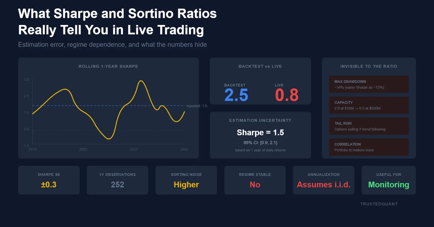
Sharpe ratio is a sample statistic with estimation error. The standard error of a Sharpe ratio estimate is approximately √((1 + 0.5 × SR²) / n), where n is the number of observations. For a strategy with a true Sharpe of 1.0 measured over one year of daily returns the standard error is around 0.07, and at a Sharpe of 2.0 it rises to around 0.11.
These error bounds matter for interpretation. A one-year track record showing a Sharpe of 1.5 is consistent with true Sharpes ranging from roughly 1.0 to 2.0 at one standard error. Two years of data helps. Three years helps more. Most allocation decisions get made with less.
def sharpe_standard_error(sharpe_estimate, n_observations):
    return np.sqrt((1 + 0.5 * sharpe_estimate**2) / n_observations)
Backtest Sharpe compounds this problem with overfitting because the reported number is the result of optimization across parameters, universe, and time period, which means the true out-of-sample Sharpe is lower and often much lower. A backtest Sharpe of 2.5 that becomes a live Sharpe of 0.8 is common.
Sortino and Downside Deviation
Sortino ratio attempts to fix the symmetry problem by replacing standard deviation with downside deviation, so only returns below some threshold contribute to the denominator. The idea is that upside volatility shouldn’t be penalized.
The fix introduces its own problems. Downside deviation is estimated from fewer observations than total volatility, so if only 40% of your returns are negative then your downside deviation estimate uses 40% of the data and estimation error increases accordingly. A Sortino ratio based on one year of daily data carries more noise than a Sharpe ratio based on the same data.
Threshold choice adds another layer of ambiguity. Using zero versus the risk-free rate versus some target return produces different numbers, and the ratio isn’t directly comparable across strategies unless the threshold is standardized, which it usually isn’t.
Distribution Shape Matters
Both ratios assume something about return distributions that often isn’t true. Sharpe works cleanly for normally distributed returns while Sortino handles asymmetry better, though both struggle with fat tails.
Positive skew with fat tails can produce a mediocre Sharpe despite excellent risk-adjusted performance because the volatility is driven by a long right tail that most investors would welcome. Negative skew with fat tails can produce a decent Sharpe that masks catastrophic risk because the left tail events haven’t happened in the sample period.
Adjustments exist for skewness and kurtosis, and they help without solving the fundamental issue since the adjustment itself is estimated from sample moments that are noisy for skewness and extremely noisy for kurtosis.
Time Period Dependence
Even with correct distributional assumptions and adequate sample size, Sharpe ratios vary dramatically across time periods for the same strategy.
A trend-following strategy might show a Sharpe of 2.0 during 2008 and 0.3 during 2012-2017. Reporting a single Sharpe across the entire period obscures this variation.
Rolling Sharpe windows reveal the instability. A strategy that looks consistent in aggregate often shows Sharpe ranging from negative to above 3.0 depending on the window, and the aggregate number averages these windows rather than reflecting a stable property of the strategy.
def rolling_sharpe(returns, window=252):
    rolling_mean = returns.rolling(window).mean()
    rolling_std = returns.rolling(window).std()
    return np.sqrt(252) * rolling_mean / rolling_std
Allocators often compare strategies by their full-period Sharpe without examining the time series of rolling Sharpe. Two strategies with identical aggregate Sharpe can have completely different profiles, with one stable across regimes and the other swinging between brilliant and terrible.
What Gets Hidden
The instability across time periods is just one dimension these ratios obscure. Several other factors that matter for allocation decisions exist entirely outside the number.
Drawdowns don’t appear in these ratios. A strategy can have a Sharpe of 1.5 with a maximum drawdown of 15% or 40%, and for most investors the drawdown matters more than the volatility.
Capacity constraints exist outside the ratio entirely. A strategy with a Sharpe of 2.0 at $10 million might have a Sharpe of 0.5 at $500 million, so the number you see is measured at a specific scale that may not match your deployment size.
Correlation with existing holdings goes unmeasured. A strategy with a Sharpe of 1.0 that’s uncorrelated with your portfolio can be more valuable than one with a Sharpe of 1.5 that’s 0.7 correlated with what you already own because portfolio-level Sharpe matters more than standalone Sharpe.
Tail risk hides behind the number entirely. A Sharpe of 1.5 generated by selling options looks the same as a Sharpe of 1.5 generated by trend following. The option seller collects premium until a tail event wipes out years of gains while the trend follower bleeds slowly and profits in dislocations. The ratio can’t distinguish between them, which is precisely when you need to look beyond it.
Practical Use
Report Sharpe and Sortino because everyone expects them. Weight them appropriately in allocation decisions, which usually means less than their prominence suggests. Look at the full return distribution, the drawdown profile, the rolling performance, and the correlation structure.
Backtest Sharpe above 2.0 often indicates overfitting, and above 3.0 almost certainly does. Live Sharpe above 2.0 sustained over multiple years is rare and usually involves leverage on a lower-Sharpe underlying strategy.
Compare ratios only within similar strategy types. A market-neutral equity strategy and a managed futures strategy have different return dynamics, so comparing their Sharpe ratios directly tells you little about which is better.
Confidence intervals help with interpretation. A Sharpe of 1.2 with a standard error of 0.3 is not meaningfully different from a Sharpe of 0.9 with the same standard error, and most performance differences between strategies fall within estimation noise.
These ratios work best for monitoring rather than selection. A strategy with a stable historical Sharpe that suddenly drops is signaling something, whether regime change, capacity constraints, or alpha decay. A strategy running two standard deviations below its historical Sharpe deserves investigation. The ratio itself won’t diagnose the cause, but the deviation from baseline tells you where to look.
This content is for educational purposes only.
Spread the word:
