

Correlation vs Cointegration and Why It Matters
Almost every pairs-trading pipeline opens the same way: building a correlation matrix over returns, keeping the pairs above some cutoff, then running a cointegration test on whatever survived. The correlation pass gets justified as a cheap first cut, since two names that barely move together day to day look like a waste of a cointegration test, yet that intuition is exactly where the edge leaks out.
The correlation filter deletes most of the pairs that carry a tradeable spread, while the ones it waves through tend to have a spread so tight that nothing is left to harvest after costs. The ordering is backwards and the damage is done before the first cointegration test runs.
The mistake is easier to see once the two statistics are kept apart, since they answer different questions about a pair.
What Correlation and Cointegration Each Measure
Correlation is a statement about returns, asking whether two assets move in the same direction on the same day on a scale from -1 to 1, while saying nothing about where the prices are. Two stocks can post a 0.9 return correlation for years even as their prices drift arbitrarily far apart, because correlation constrains the daily increments and not the levels they accumulate to.
Cointegration is a statement about levels, where two price series cointegrate when some fixed linear combination of them, the spread, is stationary, meaning it has a mean it keeps returning to and a variance that does not run off to infinity. Engle and Granger’s 1987 construction is the standard test, which regresses one log-price on the other, takes the residual and tests it for a unit root. A stationary residual ties the two prices together through an equilibrium that pulls the spread back whenever it strays, however far each price wanders on its own.
Those are different properties and neither implies the other. A pair driven by one common stochastic trend with independent short-term noise will cointegrate tightly while showing only moderate return correlation, since the shared trend governs the levels whereas the idiosyncratic noise governs the daily moves.
Run it the other way and the independence holds just as cleanly. Two names that load on the same factor each day post a high return correlation, yet if their long-run drifts differ by even a little the gap between their prices is a random walk that never reverts, so there is nothing to trade. Correlation and cointegration sit close to orthogonal, which is why using one to pre-select for the other removes the wrong pairs.
Why the Spread, Not the Correlation, Pays
A pairs trade profits from a single phenomenon: the spread reverting to its mean. However, this mean reversion relies on two properties that standard return correlation fails to capture. The spread has to be mean-reverting, which is cointegration or stationarity by another name, and it has to swing far enough that a round trip clears the bid-ask and slippage on both legs. A cointegration test measures the first property, while the second relates to the spread’s amplitude relative to costs. Correlation addresses neither.
High correlation works against the second property more often than for it, because when two assets track each other almost tick for tick the residual barely moves, leaving even a spread that passes every stationarity test too little distance between its extremes to cover the cost of trading it. The reversion is genuine and so is the relationship, yet after fees there is still nothing to collect.
Low correlation carries no such penalty, since two names with different day-to-day sensitivities can still share a long-run anchor, so their spread wanders wide and comes back, throwing off the amplitude that a spread trade needs. Those are exactly the pairs a correlation screen removes in its first pass, before cointegration is ever tested. To put numbers on what that ordering costs, it is enough to run both tests on every pair and compare what each one selects.
The Test
The panel is 242 liquid US equities and ETFs on adjusted daily closes from 2016 through 2025, all 29,161 pairs, run through a rolling walk-forward in which each step fits a two-year formation window and trades the following year out of sample, rolled to give 7 non-overlapping trading years. Formation does all the choosing, where return correlation, the Engle-Granger cointegration p-value, the hedge ratio and the Ornstein-Uhlenbeck half-life are estimated on formation data only.
The cointegration test, the half-life and the spread construction come from the pairs library used in production, so the screen here is the screen a desk would actually run, with the correlation pass and the cointegration pass amounting to two different lines of code asking two different questions:
ret_corr = np.corrcoef(np.diff(log_a), np.diff(log_b))[0, 1]

beta, alpha = np.polyfit(log_b, log_a, 1)
resid = log_a - alpha - beta * log_b
coint_p = adfuller(resid, regression="n")[1]
The first reads the daily increments, whereas the second tests whether the level gap holds together, so nothing about a high ret_corr constrains coint_p, and the panel bears that out.
Trading is deliberately plain. The spread uses the hedge ratio frozen at formation, z-scored against the formation mean and standard deviation, while a position opens when the z-score crosses 2, closes when it falls back inside 0.5, stops out past 3.5 and times out at ten half-lives. Every fill is charged 5 basis points per leg per side for spread and slippage, on both legs, at entry and exit.
Signals are causal and the spread is never re-centered on data it has not seen. The question is not whether this particular rule is a good strategy, but which pairs carry tradeable reversion and whether correlation tells you in advance.
Correlation Carries No Information About Tradeability
Across the 29,161 pairs, the rank correlation between formation return correlation and the cointegration result is +0.09, while between formation return correlation and realized out-of-sample net Sharpe it is +0.05. Both are close enough to zero that a pair’s correlation tells you essentially nothing about whether its spread cointegrates or whether it traded out of sample.
Cointegration itself is not rare here, since about a third of all pairs reject the unit-root null, and they are scattered across the whole correlation axis rather than bunched at the high end where the conventional filter looks. Figure 1 shows it directly, where the pairs that cointegrate and earned a positive net Sharpe sit at every level of correlation, with a median correlation of 0.40 that barely clears the 0.37 of the universe at large.
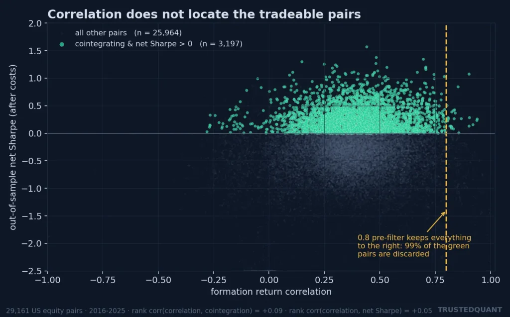
Figure 1. Out-of-sample net Sharpe against formation return correlation for all 29,161 pairs (density), with cointegrating, net-positive pairs marked. The conventional 0.8 pre-filter (dashed) sits to the right of almost all of them.
What the 0.8 Filter Throws Away
A correlation pre-filter at 0.8, a common setting, keeps just 1.1% of this universe; therefore, it discards 99% of pairs that both cointegrate and earn a positive out-of-sample net Sharpe ratio before they ever reach a cointegration test. The pairs it does keep are the wrong half of the trade, with a median formation spread of 0.040 in log terms against 0.100 for everything below the cutoff, a spread about 40% as wide.
Among the positively-correlated brackets the high-correlation pairs carry the worst median net Sharpe, well below the moderate-correlation brackets where the spread is widest. The reason is mechanical, given that a thin spread cannot cover 5 basis points a leg, so reliable reversion on a tight residual still nets a loss.
What makes the point sharper is that the reversion in those high-correlation pairs is real, since their median gross Sharpe before costs is the highest of any bin and climbs monotonically with correlation. Tighter tracking does buy cleaner mean reversion, yet it also shrinks the spread faster than it improves the reversion, so net of costs the high-correlation pairs are among the least tradeable in the universe. Gross reversion and net tradeability move in opposite directions across the correlation axis, which is the whole problem with selecting on correlation.
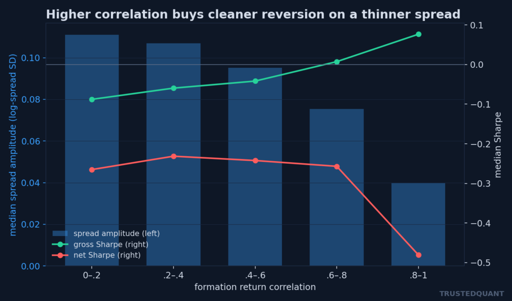
Figure 2. By correlation bracket: median spread amplitude (bars) collapses as correlation rises, while gross reversion (line) improves and net-of-cost Sharpe (line) is worst at the high-correlation end.
None of this becomes a strategy on its own, since the entry rule and the costs still decide whether a clean spread pays. What it settles is the ordering, where correlation is independent of whether a spread reverts and of how far it travels, so leading the pipeline with it discards the wide-spread cointegrating pairs and fills the book with the thin-spread ones that cannot clear costs.
A pair with a 0.3 return correlation and a wide, reliably reverting spread is the one a correlation-first screen never lets past the first step, while the tight-spread pair it keeps instead has already been compressed to the width of the bid-ask.
For the failure modes that retire these spreads in production, see Why Mean Reversion Strategies Don’t Survive Live Markets; for the construction and exit stack, see Mean Reversion in Quant Trading.
This content is for educational purposes only.
Spread the word:
