Backtesting in Quant Trading Reveals Overfitting, Bias, and False Confidence

Backtesting is the primary tool quantitative traders use to evaluate whether a strategy has an edge, and it is also the primary reason they believe in edges that do not exist. The gap between these two functions is where most capital destruction in systematic trading originates.

Most practitioners attribute this problem to overfitting: too many parameters tuned to too little data. That attribution is correct as far as it goes, which is not far enough. Overfitting is one failure mode among several, and arguably not the most dangerous one, because at least it has a name and practitioners know to look for it.

The failures that do the most damage are structural. They live in the data itself, in the assumptions the simulation framework makes about how markets work, and in the research process that produced the strategy before a single line of backtest code was written. A backtest can be methodologically clean, use proper holdout periods, avoid parameter mining, and still produce a strategy that loses money live, because the simulation never tested what the practitioner thought it was testing.

The articles linked below go deeper into each mechanism individually. What follows here is the landscape: how these failures connect, why they compound, and what separates a backtest that eliminates bad ideas from one that manufactures false conviction.

What a Backtest Actually Measures

A backtest applies a set of trading rules to historical data and records the hypothetical outcome. The output is a time series of returns, drawdowns, and performance metrics. Practitioners treat this output as evidence about the future, and the entire discipline of quantitative strategy development depends on that treatment being at least partially valid.

What a backtest actually measures is the interaction between your rules and a specific historical path, under a specific set of assumptions about execution, costs, data quality, and market structure. Change any of those assumptions and the output changes. The backtest result is a joint property of the strategy, the data, and the simulation environment, and most of the variation in backtest quality comes from the second and third components rather than the first.

Practitioners who have deployed strategies live learn to read backtests differently than those still in the research phase. A 2.0 Sharpe ratio in simulation prompts suspicion rather than excitement, because experience teaches that numbers that clean usually reflect an assumption gap rather than a genuine edge. A 0.9 Sharpe with ugly drawdowns and plausible mechanics is more credible, because the backtest is at least consistent with how markets actually behave.

The Overfitting Problem

Overfitting occurs when a model captures noise in the training data and mistakes it for signal. In backtesting, this happens through parameter optimization: testing enough combinations of lookback windows, thresholds, filters, and exit rules until the equity curve looks good. The backtest has found the specific configuration that happened to profit from the idiosyncratic features of that particular historical path. Deploy the same configuration on new data and the performance vanishes, because the idiosyncrasies were not features of the market. They were features of that sample.

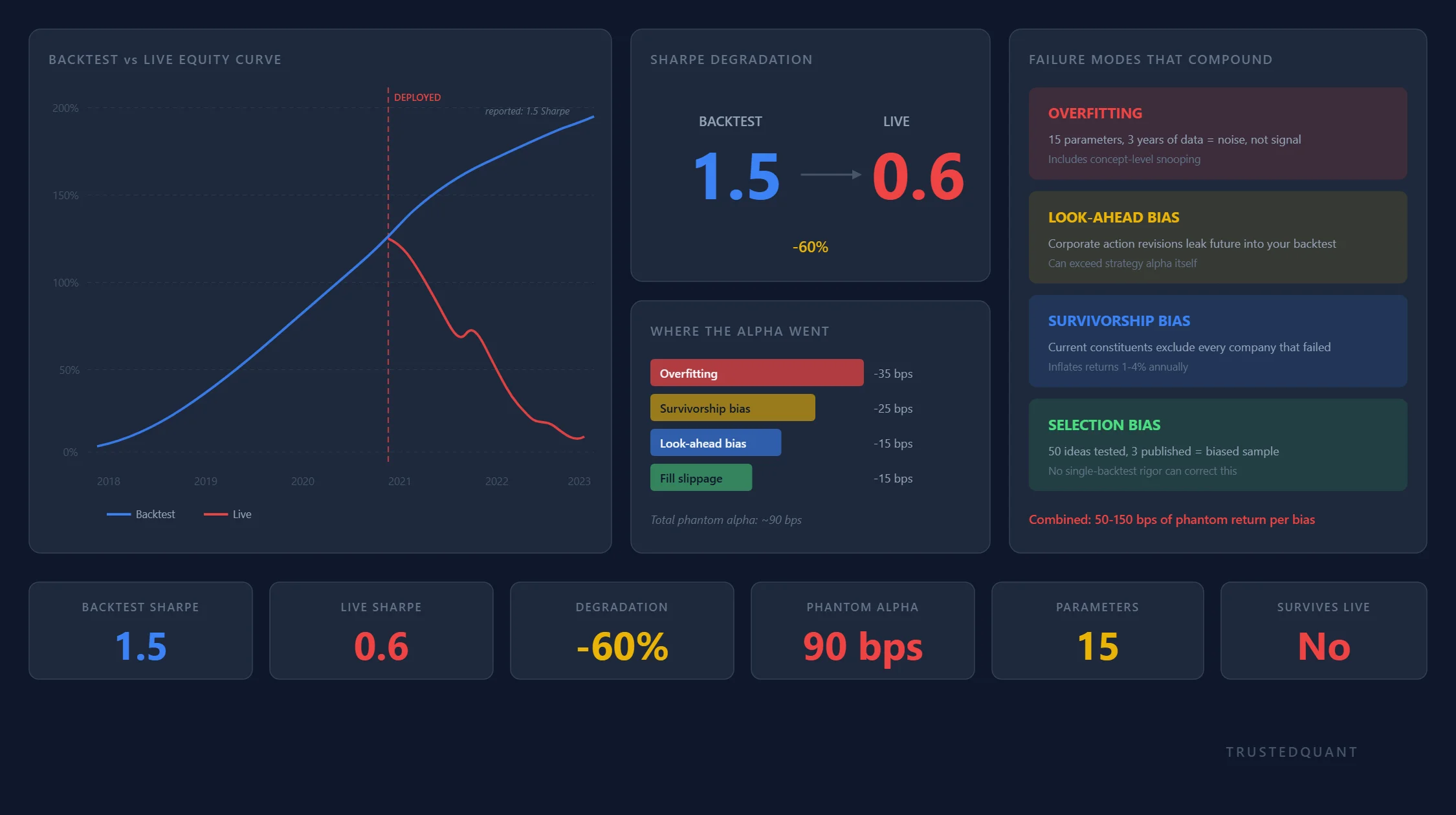
Mathematically, overfitting is well understood. Every free parameter in a strategy represents a degree of freedom that the optimizer can use to fit historical noise. Two parameters against ten years of daily data leaves enough constraint for the result to mean something, while fifteen parameters against three years can fit almost anything and means almost nothing. The ratio between degrees of freedom and independent observations is the first thing experienced researchers check, and when that ratio is unfavorable, the backtest result carries no information regardless of how impressive the equity curve looks.

What makes overfitting persistent despite being well understood is that it operates below the level of conscious parameter tuning. A researcher who tests only one parameter combination is still exposed if the strategy concept itself was selected from a larger set of ideas, each implicitly “tested” through the researcher’s prior knowledge of what has worked historically.

Consider the researcher who builds a momentum strategy in 2024. That choice implicitly draws on the knowledge that momentum has been a persistent factor for decades, which itself constitutes a form of data snooping at the concept level. Accounting for these implicit degrees of freedom is genuinely difficult, and most research processes do not attempt it.

The Bias Catalog

At least overfitting is visible when you look for it. The biases embedded in backtest data are harder to detect because they do not announce themselves through suspiciously smooth equity curves; they hide in the data pipeline itself.

Look-ahead bias enters when information that was not available at the time of a simulated trade is used to make that trade. The most common source is corporate action adjustments. A data vendor revises a historical price after a stock split, a dividend reinvestment, or a restatement, and the revised price is the one your backtest sees. Your simulation buys at a price that reflects information released weeks or months after the timestamp on the trade.

The magnitude of this bias varies by asset class and data source. In some cases it accounts for a larger share of apparent backtest alpha than the actual strategy logic, which means the strategy you think you are testing is not the strategy the backtest is running.

Testing a strategy on current S&P 500 constituents seems reasonable until you consider what the universe excludes: every company that was in the index during your test period and subsequently failed, was acquired, or was removed. Those exclusions are systematically correlated with negative returns, which means the backtest universe is artificially skewed toward winners. This is survivorship bias, and research across multiple asset classes consistently shows it inflates reported returns by one to four percentage points annually, with the effect concentrated in exactly the periods where strategy resilience matters most.

A firm that researches fifty strategy ideas and publishes the three that backtested well is presenting a biased sample even if each individual backtest was conducted properly. The published strategies were selected because they performed, and that selection process alone means the expected out-of-sample performance is lower than the in-sample results suggest. This multiple comparisons problem affects both individual researchers testing variants and the broader literature from which practitioners draw ideas, and it operates at a level that no amount of methodological rigor within a single backtest can correct.

These biases compound. A backtest that uses survivorship-biased data, conducts the test on a concept selected from prior knowledge, and fills trades at prices that incorporate future adjustments can show strong performance even when the underlying strategy has no edge at all. Each bias alone might account for 50 to 150 basis points of phantom return. Together they can fabricate an entire track record.

Why Good Backtests Still Fail Live

A backtest can avoid overfitting, use survivorship-free data, handle corporate actions correctly, and still produce a strategy that underperforms in production. The remaining gap comes from simulation assumptions that are reasonable in isolation and wrong in combination.

Fill assumptions account for most of it. A backtest that assumes you can buy at the historical close is assuming you can participate in the closing auction at exactly the printed price, with no market impact, no partial fills, and no competition from other algorithms targeting the same signal at the same time. For liquid large-cap equities in moderate size, this assumption is close enough. For anything else, the gap between assumed fills and realized fills erodes returns in proportion to the strategy’s turnover and the breadth of the universe.

Transaction costs follow a similar pattern. Commissions, spread crossing, market impact, and the opportunity cost of unfilled orders all contribute, and most backtests model only the first two. Market impact in particular is nonlinear, regime-dependent, and correlated with the signal itself, because the same conditions that generate a trading signal often generate the same signal for other participants, which means the market is moving against you before you finish executing. Modeling this accurately requires data and infrastructure that most research environments do not have.

Execution timing compounds both problems. A strategy that generates signals at the daily close and assumes execution at the next open is implicitly assuming overnight risk is free, that the opening price reflects the prior day’s information set, and that no material events occur between signal generation and execution. Each of these assumptions fails regularly enough to matter for any strategy running at scale.

Cumulatively, a backtest showing a 1.5 Sharpe ratio might deliver 0.6 to 1.0 live. That degradation is normal, and experienced practitioners budget for it by requiring backtest performance to clear a much higher bar than their target live performance. A strategy that barely justifies its costs in simulation has no chance in production.

Further Reading

This page is an anchor. The articles below go deeper into each mechanism, with code where it serves as evidence and operational detail where it changes how you build.

• Why Backtests Break in Live Trading: The structural mechanisms behind backtest-to-live degradation.
• What Makes a Strategy Survive Out of Sample: What distinguishes strategies that hold up from those that don’t.