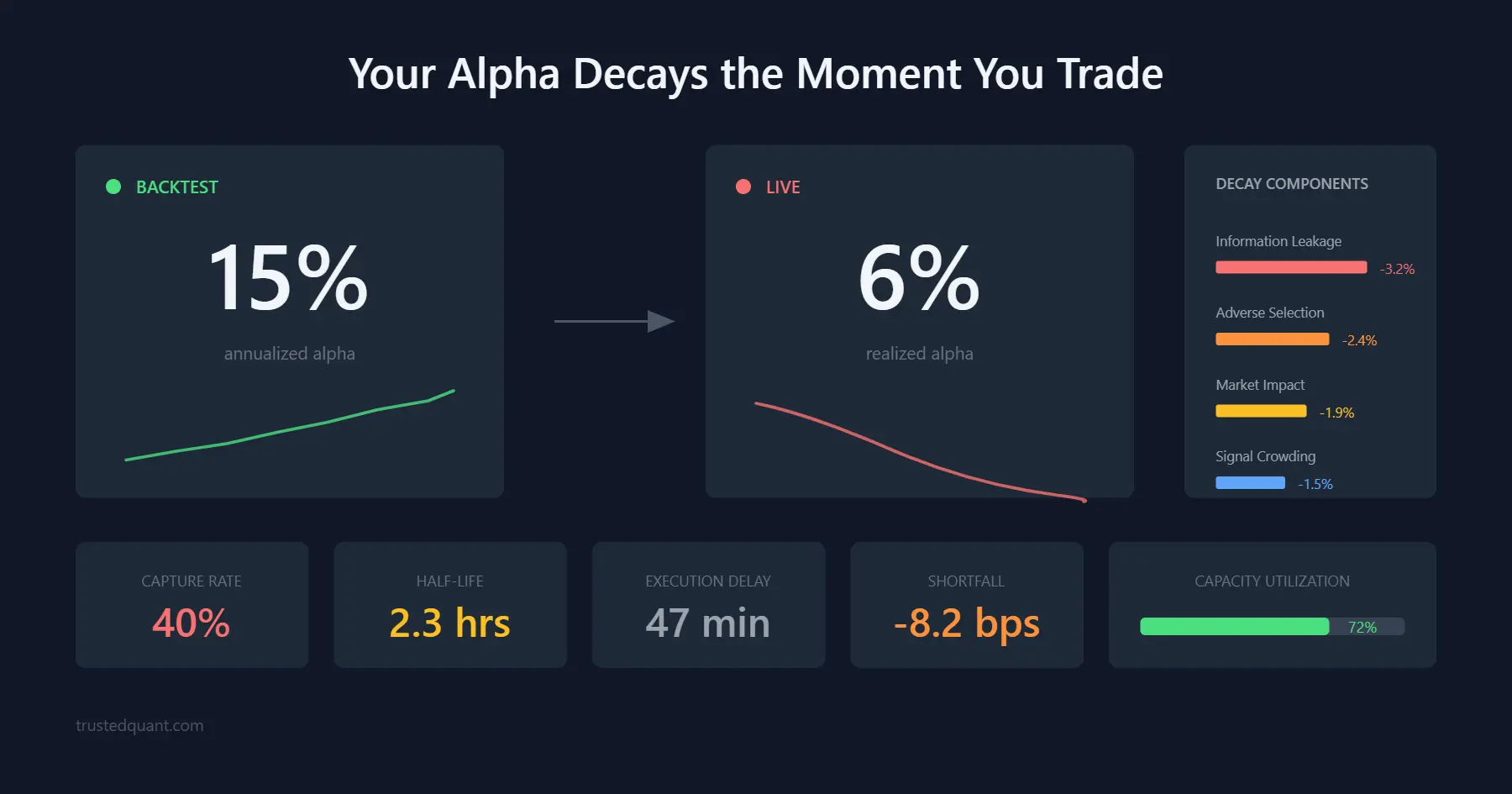
Your Alpha Decays the Moment You Trade

A backtest shows 15% annualized returns while live trading delivers 6%, even though nothing breaks and the signal captures a real regularity with fills coming in close to arrival price. The strategy underperforms persistently from the first day of production because backtests measure a signal’s predictive power in a market that has no awareness of your presence, while live trading measures what remains after the market responds to you being there.

The Backtest Runs Without You In It

Running a simulation means replaying historical prices and marking fills at the close in a market that has no idea your signal exists. It doesn’t exist yet. You build it later on data generated by other participants trading for other reasons, so the prices you see reflect a world where your strategy never acted.

Going live changes these conditions because you now submit orders based on the same signal while participating in price formation. Your bid tells the market someone wants to buy here and your offer tells someone wants to sell, so order flow carries information that gets incorporated into prices before you finish trading.

A limit order to buy at 50 communicates that someone with capital believes the asset is worth at least 50, and market makers see that signal clearly. When buyers of this size in this name at this time of day have historically been right, the market adjusts before you get filled. When they have historically been wrong, you get filled immediately because the other side knows something you don’t.

Production fills are therefore the ones the market is willing to give you conditional on everything else it knows at that moment, and execution risk arises when that conditioning works against you.

Market Impact Transfers Your Edge

Most practitioners treat this cost as a tax where you want to buy, you push the price up, and you pay a few basis points that get added to the transaction cost line. Treating impact as friction misses the economic mechanism underneath since the price moves because your order reveals information and the market prices it in.

The cost represents a transfer of value from your edge to the participants who detect your intent.

The square-root law describes the mechanical relationship where price impact scales with the square root of participation rate, so trading 1% of daily volume costs X while trading 4% costs 2X. Useful for estimation, but the formula obscures why you pay in the first place. You pay for adverse selection, which is the systematic tendency for fills to arrive at prices unfavorable to future returns.

Permanent price impact reflects this information transfer directly. Temporary impact from spread widening during execution partially reverses when you finish, but permanent impact never reverts because the market has incorporated what your trade reveals into the new equilibrium price. When you buy because you believe the price will rise and you turn out to be right, the price has already moved because your buying tells the market you think it will, so the edge you identify gets priced in through the act of expressing it.

Research on institutional order flow confirms this dynamic. Di Mascio, Lines, and Naik track post-trade alpha for fund managers and find it averages 30-40 basis points in the first month after purchase before decaying to zero by month twelve. Managers keep buying in small increments as long as the alpha persists, and their continued buying is part of what makes it disappear because the signal remains valid while the market simply learns from watching them trade.

Consistent correctness accelerates this learning because a signal that is reliably right trains the market to front-run your footprint. You become a source of information for your counterparties, and they charge you for it through the fills they are willing to give.

How Alpha Fades Over Time

Since the decay happens gradually rather than instantly, you can measure its rate to learn how much of your edge survives the transition from simulation to production. Take a signal that fires at market close and measure the return you would capture if you executed at the close versus at the next open versus midday the following day. Plotting captured return against execution delay produces your signal’s half-life curve.

def measure_decay(signal_times, signals, prices, delays, hold=1):
    captured = []
    for delay in delays:
        rets = [(prices[t + delay + hold] / prices[t + delay] - 1) * signals[t]
                for t in signal_times]
        captured.append(np.mean(rets))
    return delays, captured

def measure_decay(signal_times, signals, prices, delays, hold=1):
    captured = []
    for delay in delays:
        rets = [(prices[t + delay + hold] / prices[t + delay] - 1) * signals[t]
                for t in signal_times]
        captured.append(np.mean(rets))
    return delays, captured

Steep decay in the first minutes indicates others are trading the same information faster, which means the signal has value but you lack the infrastructure to capture it before competitors do. A curve that flattens over hours tells you the alpha persists long enough for realistic execution, so you have room to trade without losing the entire edge to faster participants. When the curve stays flat from the start, the signal may be robust to timing in ways that suggest a slower-moving inefficiency worth exploring further.

The decay profile also changes with scale. Running the same analysis at different position sizes reveals where your capacity ceiling sits because at some threshold the curve steepens as larger orders leak more information, which causes alpha to decay faster and marks the point where your footprint becomes legible enough for others to trade against.

Most daily signals show steep early decay where alpha measured on end-of-day bars has substantially dissipated by the time a realistic execution window passes. Maven Securities quantifies this cost by finding alpha decay runs 5.6% annualized in the US and 9.9% in Europe while increasing roughly 36 basis points per year as more capital chases the same signals with faster infrastructure.

Understanding the Live-Backtest Gap

Understanding the gap between backtest and live performance is where the real work begins because backtests measure a ceiling representing the maximum alpha available if you could trade without moving prices, without revealing information, and without competing against others running similar signals, making that ceiling a theoretical bound rather than an expected return. Execution costs sit at the center of what separates that bound from reality.

Raw shortfall measured as arrival price versus fill price and aggregated across trades provides the starting point, but a strategy with high shortfall might still be profitable if the alpha is large enough while a strategy with low shortfall might be worthless if the alpha is thin.

What matters is shortfall relative to expected edge and how that ratio changes under different conditions, because those changes reveal the mechanism eating your returns.

When shortfall rises as signal strength increases, the market has learned to read your urgency. Strong signals should capture more alpha, so the inversion means your execution pattern itself has become tradeable information. Someone on the other side recognizes that your speed or size correlates with conviction and positions accordingly, which means the fix requires breaking those patterns by randomizing timing and varying venues until your urgency no longer telegraphs your confidence.

The same diagnostic logic applies to position size. As you scale up, shortfall should increase according to the square-root law since larger orders move prices more. When shortfall grows faster than that relationship predicts, the market sees your full size before you finish executing and adjusts prices in anticipation, so you have hit your capacity ceiling where information leakage exceeds the edge you are trying to capture. Scaling further destroys more alpha than it adds.

A different pattern emerges when shortfall stays stable but realized alpha declines over months or years, which shows that the execution is working as designed. The shrinking returns must therefore originate in the signal itself losing predictive power as others find the same edge and their collective trading arbitrages away the returns until the market incorporates the pattern permanently.

Most practitioners fail to measure the gap with enough granularity to see which mechanism is operating. They observe underperformance and blame market conditions and keep running the same strategy hoping it reverts, even though the gap contains the information needed to diagnose what is actually happening. It tells you how the market responds to your presence and how your footprint reads to other participants and whether your edge is intact or eroding.

Backtests show you what is there. Live trading shows you what remains after you arrive to collect it, and that remainder starts shrinking the moment you trade.