
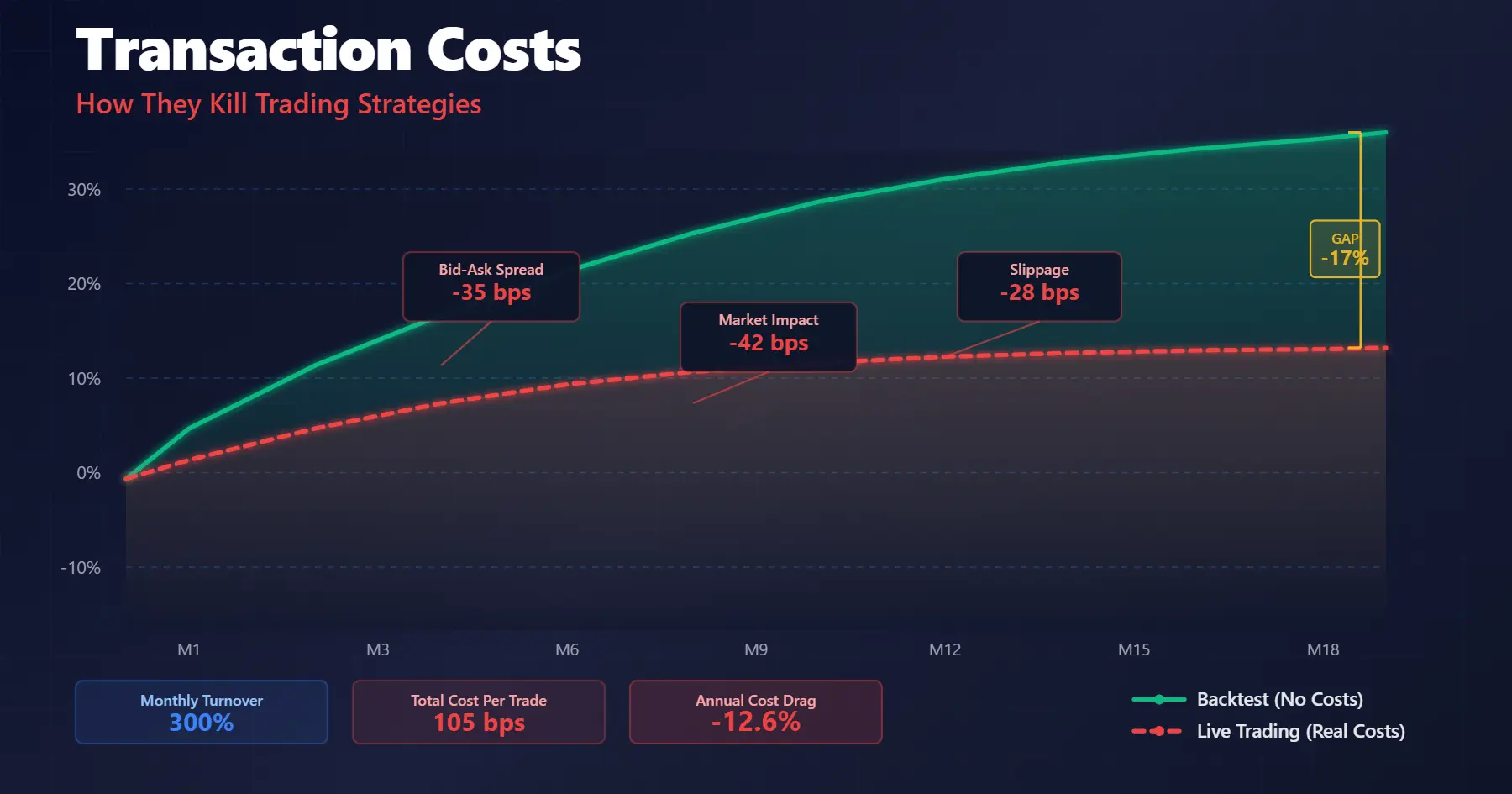
Your Transaction Costs Are Higher Than Your Model Says
Every quant shop has a cost model, and most of them are wrong in the same ways. The errors aren’t in the calibration or the parameter estimates but in the structure of the model itself, in assumptions that seemed reasonable when the model was built and have never been revisited since.
A cost model that’s wrong by 5 basis points doesn’t sound like much. At 200% annual turnover that’s 20 basis points of annual drag, and at 500% turnover it’s 50 basis points. The gap between your backtest and your live performance often lives entirely in this structural error, compounding quietly trade after trade.
The Independence Assumption
Standard cost models treat each trade as an isolated event. You estimate spread cost, add market impact, maybe include a timing component, and sum them up. The model assumes your 10:00 AM trade and your 10:15 AM trade are independent draws from the same cost distribution.
In reality, they aren’t. Your trades are correlated with each other and with everyone else’s trades. A momentum signal that fires for you fires for others running similar strategies, so you aren’t trading into average liquidity but into liquidity that’s already being consumed by correlated flow.
The independence assumption breaks hardest exactly when it matters most. On days when your signal is strongest the crowding is worst, and the cost model sees high conviction and recommends larger size while the market sees concentrated flow and charges you for it.
March 2020 made this visible. Strategies that modeled costs independently saw realized costs 3-5x higher than predicted during the second and third week of March. The models weren’t miscalibrated but structurally incapable of capturing what happens when everyone runs for the exit simultaneously.
The Linearity Assumption
The independence problem compounds when cost models also misspecify how impact scales with size.
Most cost models treat market impact as scaling linearly with trade size, or at best with the square root of trade size. The square-root model has academic pedigree and fits aggregate data reasonably well while failing precisely where accuracy matters.
def standard_impact(size, adv, volatility):
    participation = size / adv
    return 0.1 * volatility * np.sqrt(participation)
This function tells you that doubling your trade size increases impact by 40%. Empirically the relationship is closer to a power law with an exponent around 0.6, meaning doubling size increases impact by 50%. The gap seems small until you’re trading 5% of ADV and the model understates your cost by 30 basis points.
The deeper problem is that impact isn’t a smooth function at all but jumps at liquidity boundaries. When your order exhausts the displayed depth at a price level you pay a discrete penalty to access the next level, and these discontinuities don’t appear in any smooth functional form.
Real impact also depends on the state of the book when you arrive, which depends on what happened in the minutes before you arrived, which depends on flow you can’t observe. The model treats impact as a function of your trade size and some market characteristics when impact is actually a function of the entire recent history of order flow, most of which you don’t have access to.
The Stationarity Assumption
Even a model that correctly captures correlated flow and nonlinear scaling will fail if the parameters it learned no longer apply.
Cost models are calibrated on historical data, typically several months of execution records. The calibration assumes the cost-generating process is stationary, that the relationships estimated from February through July will hold in August.
Liquidity regimes shift. A stock that trades 5 million shares daily with tight spreads can become a 2 million share stock with wide spreads after index rebalancing or a change in analyst coverage. The cost model doesn’t know this happened and keeps using parameters from the old regime.
Volatility clustering creates a subtler form of non-stationarity. Your cost model might correctly estimate that volatility increases impact, but what it misses is that volatility tomorrow is correlated with volatility today. A shock to volatility persists, and your model keeps using yesterday’s volatility estimate while the market has already moved on.
The calibration window itself introduces bias. Calibrate on calm periods and you underestimate crisis costs. Calibrate on volatile periods and you overestimate costs during normal conditions, leaving money on the table by trading too passively. There’s no neutral window because the process you’re trying to estimate isn’t stationary.
The Symmetry Assumption
Even if you account for correlated flow, nonlinear scaling, and regime shifts, assuming symmetry between buying and selling still introduces a source of systematic error because standard models treat spread cost as half the spread and impact as a function of absolute trade size rather than signed trade size.
In practice, markets are far from symmetric. Selling into a falling market costs more than selling into a rising one at the same volatility level, while the order book reacts unevenly, with bid and ask depth responding differently to identical information. Short-sale constraints further amplify this asymmetry by limiting how quickly selling pressure can be expressed, so the true cost of trading depends on both direction and market context rather than just size.
Adverse selection introduces another asymmetry that most models ignore entirely. When your limit order fills quickly it usually means someone with better information was eager to trade against you, so the fill itself is a signal that you’re on the wrong side. Your cost model records the fill as a success at low spread cost while the true cost includes the subsequent adverse price movement, which averages 5-15 basis points within minutes for immediately filled orders.
The model sees a cheap fill. The P&L sees a position that’s underwater before you’ve finished blinking.
What Breaks When the Model Is Wrong
These structural errors don’t just add noise to your cost estimates but systematically bias your decisions in ways that compound over time.
Position sizing depends on cost estimates. If your model understates costs during high-conviction periods because it ignores crowding then you systematically oversize exactly when you should be more cautious, which means the positions that hurt you most are the ones where you had the highest confidence.
Rebalancing frequency depends on cost estimates. If your model underestimates spread costs in less liquid names then you rebalance them too often, and each rebalance destroys more value than your model predicts until the quarterly review shows persistent underperformance in the small-cap sleeve that nobody can explain.
Strategy selection depends on cost estimates. A backtest with a structurally flawed cost model will overstate the performance of high-turnover strategies and understate the performance of patient strategies, so you end up allocating capital to strategies that looked good in simulation and bleed in production.
The feedback loop is slow and noisy. By the time you’ve accumulated enough live trading data to see the systematic bias you’ve been paying the tax for months.
Building Less Wrong Models
Eliminating these structural flaws entirely isn’t possible because markets are too complex and too adaptive for any static model to capture them fully. What you can do is understand where your model is most likely to fail and build monitoring around those failure modes.
Track realized costs against predicted costs segmented by signal strength. If realized costs consistently exceed predictions when conviction is high then your model is missing crowding effects. The correlation between prediction error and signal strength is more diagnostic than the average prediction error.
Track cost prediction errors across volatility regimes separately. A model that’s well-calibrated on average might be 30% wrong in high-volatility periods, and the average looks fine because high-volatility periods are rare while the P&L impact is concentrated in exactly those periods.
Track the autocorrelation of prediction errors. If today’s error predicts tomorrow’s error then your model is missing regime shifts. Independent errors suggest the model is capturing the structure correctly even if the parameters are noisy, while correlated errors suggest something structural is wrong.
def model_diagnostic(predicted_costs, realized_costs, signal_strength, volatility_regime):
    errors = realized_costs - predicted_costs

    corr_with_signal = np.corrcoef(errors, signal_strength)[0, 1]
    error_autocorr = np.corrcoef(errors[:-1], errors[1:])[0, 1]

    high_vol_bias = errors[volatility_regime == 'high'].mean()
    low_vol_bias = errors[volatility_regime == 'low'].mean()

    return {
        'signal_correlation': corr_with_signal,
        'error_persistence': error_autocorr,
        'high_vol_bias': high_vol_bias,
        'low_vol_bias': low_vol_bias
    }
The output tells you which structural assumption is hurting you most. Signal correlation points to independence failures. Error persistence points to stationarity failures. Regime-specific bias points to calibration window problems.
None of this makes the model correct. It tells you how the model is wrong, which lets you make less bad decisions with it. A cost model you understand is more valuable than a sophisticated one you trust blindly.
The Honest Implication
Every backtest you’ve ever run used a cost model with these structural flaws. The strategies that looked best were often the ones where the model’s blind spots aligned most favorably with the strategy’s trading pattern, meaning high-turnover strategies in correlated names, sized up during high-conviction periods, tested on calm historical windows.
The gap between backtest and live performance isn’t random. It’s the market charging you for assumptions you didn’t know you were making.
This content is for educational purposes only.
Spread the word:
